Why Does an OFDM Signal Have a Rayleigh Distribution?

A complicated communication signal can sometimes be understood using surprisingly elementary mathematics.

Consider a large number of vectors of length 1 pointing in random directions. Add them together. What can we say about the length of the resulting vector?

This seemingly geometric probability problem leads directly to a standard mathematical model for OFDM (Orthogonal Frequency-Division Multiplexing), a technique used in modern digital communication.

The path is beautiful:

random phases → sine and cosine → Central Limit Theorem → two-dimensional Gaussian → Rayleigh distribution.

Step 1: Add Random Unit Vectors

Suppose that

θ_{1}, θ_{2}, \dots, θ_{N}

are independent random angles uniformly distributed between 0 and $2 π$ .

The corresponding unit complex numbers are

e^{i θ_{k}} = cos θ_{k} + i sin θ_{k} .

Now add all of them:

Z = \sum_{k = 1}^{N} e^{i θ_{k}} .

Separating the real and imaginary parts gives

Z = X + i Y,

where

X = \sum_{k = 1}^{N} cos θ_{k}, Y = \sum_{k = 1}^{N} sin θ_{k} .

Step 2: What Is the Distribution of One Coordinate?

If $θ$ is uniformly distributed on $[0, 2 π]$ , then both $sin θ$ and $cos θ$ have density

g (x) = \frac{1}{π \sqrt{1 - x^{2}}}, - 1 < x < 1 .

This is sometimes called the arcsine distribution.

By symmetry,

E [cos θ] = E [sin θ] = 0 .

Also,

E [{cos θ}^{2}] = E [{sin θ}^{2}] = \frac{1}{2} .

Therefore each coordinate has mean 0 and variance $\frac{1}{2}$ .

Step 3: The Central Limit Theorem Appears

Now comes the key step.

Both $X$ and $Y$ are sums of many independent random variables.

When $N$ is large, the Central Limit Theorem tells us that these sums are approximately normally distributed:

X \approx N (0, \frac{N}{2}),

Y \approx N (0, \frac{N}{2}) .

In other words, the endpoint of our random walk is approximately described by a two-dimensional Gaussian distribution centered at the origin.

Step 4: How Far Are We from the Origin?

The amplitude of the complex sum is

R = | Z | = \sqrt{X^{2} + Y^{2}} .

So we have reached a purely geometric question:

If a point has two independent Gaussian coordinates, what is the distribution of its distance from the origin?

The answer is the Rayleigh distribution.

Since each coordinate has variance $\frac{N}{2}$ , the approximate density of $R$ is

f (r) \approx \frac{2 r}{N} \exp (- \frac{r^{2}}{N}), r \geq 0 .

This formula is important to interpret correctly. For a finite number of random unit vectors it is generally not the exact distribution. It is the large- $N$ approximation produced by the Central Limit Theorem.

A Shorter Derivation of the Rayleigh Formula

There is also a beautiful geometric way to obtain the density.

For large $N$ , the joint density of $(X, Y)$ is approximately

p (x, y) = \frac{1}{π N} \exp (- \frac{x^{2} + y^{2}}{N}) .

This density depends only on the distance from the origin.

A thin circular ring of radius $r$ and thickness $d r$ has area approximately

2 π r d r .

Multiplying the two-dimensional density by this ring area gives

\frac{1}{π N} \exp (- \frac{r^{2}}{N}) \cdot 2 π r d r .

Therefore,

f (r) = \frac{2 r}{N} \exp (- \frac{r^{2}}{N}) .

So the factor $r$ in the Rayleigh distribution has a simple geometric origin: circles become longer as their radius increases.

What Does This Have to Do with OFDM?

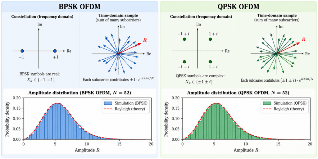
An OFDM time-domain sample is produced by an inverse discrete Fourier transform. It therefore involves adding many complex contributions having different phases.

This suggests viewing the sample, in a simplified model, as a sum of many complex vectors.

That brings us back to exactly the random-vector problem above.

An Example with 52 Active Carriers

Consider a system with 64 available carrier positions, of which 52 are nonzero: 48 data carriers and 4 pilot carriers.

The simple random-phasor model therefore suggests taking

N = 52 .

For a Rayleigh distribution with the density derived above, the expected amplitude is

E [R] = \frac{\sqrt{π N}}{2} .

For $N = 52$ , this gives

E [R] = \frac{\sqrt{52 π}}{2} \approx 6.3907 .

How Good Is the Approximation?

I originally investigated this question numerically by comparing the simple theoretical model with simulated OFDM signals.

The theoretical mean amplitude for the 52-vector model is approximately 6.3907.

A direct simulation of the random-vector model produced 6.3796.

The corresponding simulated OFDM mean amplitudes were:

Model	Mean amplitude
Rayleigh theory	6.3907
Random-vector simulation	6.3796
BPSK OFDM	6.3889
QPSK OFDM	6.4015
16QAM OFDM	6.4058
64QAM OFDM	6.3837

The agreement is remarkably good.

A complicated digital communication signal has, at least at the level of its typical amplitude, been captured by a very simple model: add 52 vectors pointing in random directions.

But What About Rare Peaks?

Matching the average is not the whole story.

For communication systems, unusually large signal peaks are important. An amplifier must be able to accommodate those peaks without severe distortion.

This is where the difference between an approximation and an exact distribution becomes important.

In the original numerical experiment, the simple theory tracked several OFDM simulations quite well at moderate thresholds. But differences appeared in the far tail of the distribution, particularly for BPSK.

For example, at a peak-to-average threshold of 12 dB, the values from that simulation were approximately

Model	Tail probability
Simple theory	4.0 × 10⁻⁶
BPSK	1.969 × 10⁻³
QPSK	9.4 × 10⁻⁵
16QAM	7.9 × 10⁻⁵
64QAM	4.0 × 10⁻⁵

This illustrates an important lesson in probability.

Two distributions can look very similar around their typical values while behaving quite differently in their extreme tails.

The Central Limit Theorem explains the center of the distribution extremely well, but rare events can require more careful analysis.

The Mathematics Behind a Communication Signal

What I like about this example is the number of mathematical ideas that meet in one problem.

We started with complex numbers:

e^{i θ} = cos θ + i sin θ .

Those became random vectors in the plane.

Their coordinates led to probability distributions.

Adding many of them brought in the Central Limit Theorem.

The resulting two-dimensional Gaussian led, through elementary geometry, to the Rayleigh distribution:

f (r) \approx \frac{2 r}{N} \exp (- \frac{r^{2}}{N}) .

And that simple formula gives a surprisingly accurate description of the amplitude of an OFDM signal.

This is a good example of why mathematical modeling is so useful: the real system may be complicated, but sometimes the right simplified model exposes the mathematics underneath it.

Where the Gaussian Function Enters the Story

The Rayleigh distribution in OFDM is closely connected to Gaussian random variables. When many independent contributions combine, the in-phase and quadrature components of the signal are approximately Gaussian, and their magnitude produces the Rayleigh distribution.

At the heart of the Gaussian distribution is the remarkable function $e^{- x^{2}}$ . Its integral over the real line cannot be evaluated by finding an ordinary elementary antiderivative. Yet there is a beautiful way to compute it by moving from one dimension to two.

Continue exploring: The Gaussian Integral and Beyond: From e^(-x²) to a Family of Integrals

Why Does an OFDM Signal Have a Rayleigh Distribution?

Step 1: Add Random Unit Vectors

Step 2: What Is the Distribution of One Coordinate?

Step 3: The Central Limit Theorem Appears

Step 4: How Far Are We from the Origin?

A Shorter Derivation of the Rayleigh Formula

What Does This Have to Do with OFDM?

An Example with 52 Active Carriers

How Good Is the Approximation?

But What About Rare Peaks?

The Mathematics Behind a Communication Signal

Where the Gaussian Function Enters the Story

More posts

How the Ancient Greeks Summed Infinite Series Without Calculus

Kepler’s Laws: How Calculus Explains Planetary Motion

Bézier Curves: How Four Points Create Beautiful Shapes

The Geometry of a Tetrahedron: From Pythagoras to Vector Identities

Leave a Reply Cancel reply