Blog

  • How the Ancient Greeks Summed Infinite Series Without Calculus

    Can infinitely many pieces have a finite total area? The Greeks approached this question through geometric exhaustion. Archimedes proved that a parabolic segment has four-thirds the area of its largest inscribed triangle. Here we explain the geometry with modern notation, clearly distinguishing ancient arguments from modern illustrations.

    1. Zeno and infinitely many steps

    Travel half a unit, then a quarter, then an eighth, and so on. The infinite subdivision raises Zeno’s famous question: can infinitely many stages have a finite total?

    12+14+18+⋯=1
    Zeno’s successive halfway distancesA segment from zero to one marked at one half, three quarters, seven eighths, and fifteen sixteenths, with arrows indicating successive travel distances.01/23/47/811/21/41/8The successive distances shrink, while their total approaches 1.
    Figure 1. Zeno’s successive halfway distances. This is a modern diagram of the ancient philosophical problem.

    After n steps the distance left is 1/2n. It tends to zero, although no finite step reaches the endpoint.

    2. A square proves a geometric series

    Partition a unit square into vertical strips of widths 1/2, 1/4, 1/8, … . The strip areas have exactly these values.

    Geometric series filling a squareA square divided into vertical strips of widths one half, one quarter, one eighth, one sixteenth and progressively narrower widths. The remaining unfilled strip tends to zero.1/21/41/8The entire square has area 1.Each new strip occupieshalf the remaining area.No finite step fillsthe entire square.The uncovered areatends to zero.
    Figure 2. Successive strips fill the unit square in the limit. Each new strip is half the remaining width.
    Sn=1−12n

    Since the unfilled strip has area 1/2n, its area approaches zero. The same argument gives the general geometric sum when 0 < q < 1:

    1+q+q2+⋯=11−q

    The colored-square construction and modern series notation are teaching devices, not a reconstruction of a particular surviving ancient proof.

    3. Archimedes’ quadrature of the parabola

    Consider the region between y = 1 − x² and the chord from (−1,0) to (1,0). Its largest inscribed triangle has vertices (−1,0), (0,1), (1,0), and area T = 1.

    Archimedes’ parabolic segment with generations of trianglesThe parabolic arc from minus one to one above its horizontal chord. A large blue inscribed triangle is followed by two orange triangles and four smaller green triangles filling the remaining curved regions.(0, 1)(-1, 0)(1, 0)Area TTotal T/4Total T/16Successive triangle generations fill the parabolic segment.
    Figure 3. The blue triangle has area T. The orange pair totals T/4, and the green group totals T/16. Later generations continue the same pattern.

    Why does every generation shrink by a factor of four?

    The next triangle on the left has vertices (−1,0), (0,1), and (−1/2,3/4). The determinant formula gives area 1/8. The symmetric right triangle also has area 1/8, so their combined area is T/4.

    For any two points of the parabola with x-coordinates a and b, the tangent parallel to their chord occurs at x = (a+b)/2. A determinant calculation gives the inscribed triangle area:

    T(a,b)=b−a38

    Halving the interval [a,b] produces two child triangles, each with 1/8 of its parent’s area. Thus their combined area is 1/4 of the parent’s area. This repeats at every stage.

    A=T(1+14+116+⋯)=4T3

    Since T = 1 in our example, the curved segment has area 4/3. Modern integration confirms that the integral of 1 − x² from −1 to 1 equals 4/3.

    4. Why exhaustion proves the result

    Archimedes needed more than an attractive pattern: he had to show that the remaining curved slivers could have arbitrarily small total area. Let Sn denote the first n+1 generations. The finite geometric sum is

    Sn=4T3(1−14n+1)

    Each remaining parabolic segment fits inside a parallelogram of twice the area of its largest inscribed triangle. Thus, after n generations, the total leftover area Rn obeys:

    0≤Rn≤2T4n+1

    The right side tends to zero, proving that the triangles exhaust the parabolic segment. This is a modern remainder-bound presentation of the geometric reasoning.

    Method of exhaustion boundsA number line with the partial sums S n below four thirds, and shrinking remainders, illustrating that the sum approaches four thirds.S₀ = 1S₁ = 5/44/3Remainder decreases to zero0Illustration is schematic; marks are not to scale.
    Figure 4. The finite areas approach 4T/3 while the leftover area becomes arbitrarily small. Schematic, not to scale.

    5. Another area series: thirds

    A rectangle of area 1/2 can be partitioned into strips with areas 1/3, 1/9, 1/27, … by taking two-thirds of what remains at each step. Hence

    13+19+127+⋯=12

    6. Why the harmonic series behaves differently

    Not every infinite collection of positive areas has a finite sum. Group the harmonic series as 1; 1/2; (1/3 + 1/4); (1/5 + ⋯ + 1/8); and so on. Every group after the first totals at least 1/2. Thus the partial sums grow without bound. Rectangles of width 1 and heights 1, 1/2, 1/3, … have unbounded combined area.

    7. From Greek geometry to calculus

    The method of exhaustion anticipates integration: approximate a curved region with simple shapes, then control the error. The Greeks did not write modern limit or integral notation, but their finite geometric comparisons could establish exact areas.

    Discovery problems

    1. Give a geometric proof that 1/3 + 1/9 + 1/27 + ⋯ = 1/2.

    2. For a starting triangle of area T, find the sum of the first n+1 Archimedean generations and bound the remainder.

    3. For the segment under y = 9 − x² above the x-axis, find the largest inscribed triangle area and then the curved area. Check by integration.

    4. Show geometrically by grouping that the harmonic series diverges, and explain why this does not contradict the square partition.

    Solutions (click to reveal)

    Solution 1

    Begin with a rectangle of area 1/2. Take two-thirds of its area, then two-thirds of the remainder, repeatedly. The removed areas are 1/3, 1/9, 1/27, … . The remainder after n steps is (1/2)(1/3)n, which tends to zero.

    Solution 2

    Sn = (4T/3)(1 − 4−(n+1)). The unfilled area is at most 2T/4n+1, by the enclosing-parallelogram bound. It tends to zero.

    Solution 3

    The endpoints are (−3,0), (3,0) and the apex is (0,9). The triangle area is T = (1/2)(6)(9) = 27. Archimedes gives 4T/3 = 36. Integrating 9 − x² from −3 to 3 also gives 36.

    Solution 4

    Group 1/2; (1/3+1/4); (1/5+⋯+1/8); and so on. Every group contains twice as many terms as the previous, each at least half the preceding minimum, so each group totals at least 1/2. The area grows without bound, unlike the square partition whose total is at most 1.

    Historical sources

    • Archimedes, Quadrature of the Parabola, especially Propositions 21–24.
    • Euclid, Elements, Book XII.
    • Thomas L. Heath, The Works of Archimedes (1897 translation and commentary).

    Historical note: The modern algebra, colored diagrams, and integration checks are explanatory additions, not verbatim ancient arguments.

    Archimedes used geometry to evaluate infinite sums long before the development of calculus. Centuries later, mathematicians discovered remarkable geometric and analytic methods for evaluating more complicated series. Explore one such example in our article on the Basel problem and its solution using a double integral .

    The relationship between infinity and geometry continues to produce surprising results. For example, a surface can have infinite area while enclosing a finite volume. Discover this phenomenon in Gabriel’s Horn .
  • Kepler’s Laws: How Calculus Explains Planetary Motion

    Why do planets move faster near the Sun? Why do they sweep out equal areas in equal times? And why does a planet farther from its star take longer to complete an orbit? These questions connect geometry, derivatives, Newton’s laws, and a remarkably simple relationship between orbital size and orbital period.

    Model and notation. We use Newtonian gravity and first treat a planet whose mass is negligible compared with its star’s mass M. Write G for the gravitational constant and μ = GM for the gravitational parameter. For two bodies of comparable mass, replace GM with G(M + m) in the relative-orbit formulas. We assume an ideal isolated two-body system unless stated otherwise.

    1. Three laws, one mathematical story

    First law: A planet follows an ellipse with the Sun at one focus. Second law: The line from the Sun to the planet sweeps out equal areas in equal times. Third law: For planets orbiting the same star, the square of the orbital period is proportional to the cube of the semimajor axis.

    Let the focal distance be c. The eccentricity is e = c/a, with 0 ≤ e < 1 for an ellipse. The familiar circle is the special case e = 0. We will derive all three laws from a central inverse-square force.

    2. Newton’s inverse-square force and the orbit equation

    The acceleration of a planet at position vector r relative to the star is directed toward the star:

    d2𝐫/dt2=−GMr3𝐫

    Here r without boldface is the distance to the star. In plane polar coordinates, the radial and transverse components of acceleration are

    ar=r″−rθ′2,aθ=rθ″+2r′θ′

    Primes in this section mean derivatives with respect to time. Since gravity has no transverse component,

    d/dt(r2θ′)=0

    Therefore h = r²θ′ is constant. To derive the orbit shape, set u(θ) = 1/r. The radial equation becomes the Binet equation:

    d2dθ2u+u=μh2

    To see this, note that r′ = −h uθ and r″ = −h²u²uθθ, while rθ′² = h²u³. Substituting into the radial equation and dividing by −h²u² gives the displayed equation. Its general solution is

    u(θ)=μh2[1+ecos(θ−θ0)]

    Choose θ = 0 in the perihelion direction, so θ₀ = 0. Inverting gives the polar conic equation:

    r=p1+ecosθ p=h2μ

    For 0 ≤ e < 1, this is an ellipse. Thus Newton’s inverse-square force yields Kepler’s First Law for bound noncircular and circular orbits. The same equation also describes parabolic or hyperbolic paths when e ≥ 1.

    3. Kepler’s Second Law: why equal areas take equal times

    Let v = dr/dt. Because gravitational acceleration is parallel to r,

    ddt(r×v)=drdt×v+r×dvdt=v×v+r×a=0.

    The vector r × v is constant. Its magnitude h equals r² dθ/dt, the specific angular momentum. A narrow sector of angle dθ has area dA ≈ ½r²dθ. Taking the limit,

    dAdt=12r2dθdt=h2

    Therefore the area swept out per unit time is constant. Near perihelion, r is small and the angular speed dθ/dt = h/r² is large; near aphelion, the angular speed is smaller. This is Kepler’s Second Law.

    4. Kepler’s Third Law from the area of an ellipse

    An ellipse with semiaxes a and b has area πab. Since the radius vector sweeps out this entire area in one period T and dA/dt = h/2,

    T=2πabh

    The ellipse geometry gives b² = a²(1 − e²). The polar conic parameter p satisfies p = a(1 − e²) = b²/a. From Section 2, h² = μp, so

    h2=μb2a

    Squaring the period formula and substituting yields

    T2=4π2a3μ

    This is Kepler’s Third Law in its Newtonian form. In a two-body system with planet mass m not negligible, the more general relation is

    T2=4π2a3G(M+m)

    5. Worked example: the orbital period of Mars

    Use a new example: Mars has semimajor axis approximately 1.524 AU. Earth’s semimajor axis is approximately 1 AU, and its orbital period is approximately one year. Since both orbit the Sun, Kepler’s Third Law gives

    TMars2TEarth2=aMarsaEarth3 TMars=1.52432years≈1.881years

    Multiplying by 365.25 days per year gives approximately 687 days, consistent with Mars’s orbital period. Notice that the eccentricity does not appear: the semimajor axis, not the semiminor axis, controls the period in the ideal two-body model.

    6. Why a geostationary satellite stays over one point

    A geostationary satellite moves in a circular, equatorial, prograde orbit whose period equals Earth’s sidereal rotation period, approximately 86,164 seconds—not the 86,400 seconds of a mean solar day.

    For a circular orbit of radius r, gravity supplies centripetal acceleration:

    GMr2=v2r

    Because v = 2πr/T, solving for r gives

    r=GMT24π213

    Using Earth’s gravitational parameter GM ≈ 3.986004418 × 10¹⁴ m³/s² and equatorial radius approximately 6,378 km gives an orbital radius of about 42,164 km and an altitude of about 35,786 km above the equator. A satellite with the same period but an inclined or eccentric orbit is geosynchronous, not necessarily geostationary.

    7. Beyond Kepler: orbital energy and the limits of the model

    The specific mechanical energy (energy per unit planet mass) is

    ε=v22−μr

    For a bound Kepler ellipse, a standard consequence of the orbit equation and conservation laws is

    ε=−μ2a

    Equating these expressions gives the vis-viva equation:

    v2=μ(2r−1a)

    At perihelion r = a(1 − e), and at aphelion r = a(1 + e). Using h = rv at these turning points, where velocity is tangential,

    vperivaph=1+e1−e

    Real planetary orbits experience perturbations from other planets, nonspherical gravity fields, and relativistic corrections. Kepler’s laws remain an extraordinarily accurate first approximation, not an exact description of every real orbit.

    Discovery problems

    Try these before opening the solutions. Each problem extends one of the article’s central ideas.

    Problem 1. How much faster at perihelion?

    For an elliptical orbit of eccentricity e = 0.30, find the ratio of perihelion speed to aphelion speed. Explain your result without calculating either speed separately.

    Problem 2. A planet around a heavier star

    A planet has semimajor axis 3 AU and orbits a star of mass twice the Sun’s mass. Neglect the planet’s mass. Find its period in Earth years.

    Problem 3. Escape velocity

    Starting from conservation of mechanical energy, derive the minimum escape speed from distance R from a spherical planet of mass M. Estimate Earth’s surface escape speed using GM ≈ 3.986 × 10¹⁴ m³/s² and R ≈ 6.371 × 10⁶ m. Ignore the atmosphere and rotation.

    Problem 4. Different shapes, same period

    Two satellites orbit the same planet in ideal elliptical orbits with the same semimajor axis a but eccentricities e₁ = 0.1 and e₂ = 0.7. Prove that their periods agree, and explain why their speeds need not agree at corresponding locations.

    Solutions (open only after trying the problems)

    Solution to Problem 1

    Angular momentum per unit mass is conserved. At perihelion and aphelion the velocity is perpendicular to the radius, so rpvp = rava. Since rp = a(1 − e) and ra = a(1 + e),

    vpva=1+0.301−0.30=137≈1.857

    The planet moves about 1.86 times as fast at perihelion.

    Solution to Problem 2

    Relative to Earth’s orbit, the semimajor axis is three times as large and the central mass is twice as large. Therefore

    T21 year2=332

    Hence T = √(27/2) years ≈ 3.67 years.

    Solution to Problem 3

    At the threshold of escape, the spacecraft arrives infinitely far away with zero residual speed, so its specific mechanical energy is zero:

    vesc22−GMR=0vesc=2GMR12

    Substituting Earth’s values gives approximately 11.2 km/s. This neglects drag and Earth’s rotation.

    Solution to Problem 4

    Kepler’s Third Law gives T² = 4π²a³/(GM) for both satellites. Their shared a and M imply identical periods. But the vis-viva equation v² = GM(2/r − 1/a) shows that speed depends on the instantaneous distance r. The more eccentric orbit has a greater variation in r and therefore a greater variation in speed.

    Further connections

    Kepler’s laws are an especially useful example of how parametric curves and geometry lead to physical predictions. For another application of parametric descriptions, explore Bézier Curves: How Four Points Create Beautiful Shapes.

    Further reading: Newton, Philosophiæ Naturalis Principia Mathematica (1687); standard introductory treatments of Newtonian gravitation, central forces, and conic sections. Numerical constants above are rounded for illustration.

    Newton’s laws explain not only planetary orbits but also the motion of projectiles near Earth’s surface. For another application of vector calculus, see Projectile Motion in Three Dimensions .

    Calculus can also reveal surprising behavior in everyday mechanical systems. Explore another example in The Sliding Ladder: Does It Slide or Jump? .

  • Bézier Curves: How Four Points Create Beautiful Shapes

    How can four points create a smooth curve? Cubic Bézier curves appear in fonts, vector graphics, animation, and computer-aided design. Their geometry is controlled by just four points, yet they can bend, change concavity, and even cross themselves.

    1. Four control points and one curve

    Let P₀, P₁, P₂, and P₃ be points in the plane. For 0 ≤ t ≤ 1, define

    B(t)=1−t3P0+3t1−t2P1+3t21−tP2+t3P3

    Operations on points are interpreted coordinatewise. The curve begins at P₀ and ends at P₃. The broken line P₀P₁P₂P₃ is the control polygon; the curve need not pass through its middle vertices.

    A new numerical example

    Choose P₀=(0,0), P₁=(2,5), P₂=(6,5), P₃=(8,0). Substitution and simplification give

    x(t)=6t+6t2−4t3, y(t)=15t−15t2

    For example, at t=1/2, the point is B(1/2)=(4,15/4). The symmetry of the control points produces a symmetric arch.

    P0P1P2P3
    Figure 1. Our new example (blue) and its dashed control polygon. The middle control points guide the shape but are not on the curve.

    2. Why the curve stays in the convex hull

    The four scalar weights are (1−t)³, 3t(1−t)², 3t²(1−t), and t³. They are nonnegative for 0 ≤ t ≤ 1, and their sum is

    1−t3+3t1−t2+3t21−t+t3=(1−t+t)3=1

    Proof. By definition, a convex combination of points is a weighted sum with nonnegative weights totaling one. Every B(t) is such a combination of the four control points. Hence the entire curve lies in their convex hull—the smallest convex region containing them. This remains true even if the curve has a loop.

    3. Endpoint tangents

    Differentiate the defining polynomial and group the terms:

    B(t)′=31−t2(P1−P0)+6t1−t(P2−P1)+3t2(P3−P2)

    Consequently,

    B(0)′=3(P1−P0), B(1)′=3(P3−P2)

    Thus, whenever the respective endpoint derivative is nonzero, the tangent line at the start follows P₀P₁, and the tangent line at the end follows P₂P₃. In our example these tangent vectors are (6,15) and (6,−15). Notice that these vectors specify tangent directions, not necessarily the direction of the entire control polygon.

    4. De Casteljau’s algorithm: constructing the curve by interpolation

    For a fixed t, interpolate successively between neighboring control points:

    Qi=1−tPi+tPi+1 (i=0,1,2) Ri=1−tQi+tQi+1 (i=0,1,1) B(t)=1−tR0+tR1

    Why it works. Substitute the formulas for Q₀,Q₁,Q₂ into those for R₀,R₁, then into the last expression. Collecting the coefficients of P₀ through P₃ produces exactly the cubic Bézier formula in Section 1.

    At t=1/2, the first interpolation points are Q₀=(1,5/2), Q₁=(4,5), Q₂=(7,5/2); the next points are R₀=(5/2,15/4), R₁=(11/2,15/4). Their midpoint is (4,15/4), as expected.

    P0P1P2P3
    Figure 2. De Casteljau construction at t=1/2: orange first-stage interpolation, green second-stage interpolation, and the final black point on the curve.

    5. Can a cubic Bézier curve have a loop?

    Yes. Here is an exact construction, deliberately different from the textbook example. Consider the parametric cubic

    x(t)=(t−12)2, y(t)=(t−12)((t−12)2−116)

    At t=1/4 and t=3/4, both expressions yield the same point (1/16,0). Since the parameters are distinct, the curve crosses itself. Its Bézier control points, obtained by converting the cubic power coefficients to Bernstein form, are

    P0=(14,−332); P1=(−112,1396); P2=(−112,−1396); P3=(14,332)
    t=1/4 and 3/4
    Figure 3. An exact cubic loop. The two parameter values 1/4 and 3/4 give the same crossing point.

    6. Joining Bézier curves smoothly

    Suppose one segment ends at P₃ and the next begins at Q₀. Three commonly used continuity conditions are:

    C⁰: P₃=Q₀, so the pieces meet. G¹: their nonzero tangent vectors point in the same direction, so the tangent line has no corner. C¹: their tangent vectors are equal (for the chosen parameterization), so the first derivative is continuous.

    C1: P3=Q0, 3(P3−P2)=3(Q1−Q0)

    For a concrete S-shaped construction, take the first control polygon (0,0),(1,2),(2,2),(3,0) and the second (3,0),(4,−2),(5,−2),(6,0). Both derivatives at the join equal (3,−6), so the pieces meet with C¹ continuity. Equal tangents are stronger than merely collinear tangents.

    join
    Figure 4. Two cubic segments form an S-shaped path and meet with matching derivatives at (3,0).

    7. Curvature, inflection points, and a cubic limitation

    For a regular parametric curve B(t)=(x(t),y(t)), meaning B′(t)≠0, the unsigned curvature is

    κ(t)=|x′(t)y″(t)−y′(t)x″(t)|(x′2+y′2)32

    The numerator is the signed turning determinant. For cubic coordinate polynomials, x′ and y′ are quadratic while x″ and y″ are linear. Although the products appear cubic, their cubic terms cancel, leaving a polynomial of degree at most two. Therefore a nondegenerate regular planar cubic Bézier curve has at most two isolated interior inflection points, since changes in signed curvature can occur only at zeros of this quadratic.

    In our arch example, x′=6+12t−12t² and y′=15−30t, while x″=12−24t and y″=−30. Hence

    x′y″−y′x″=−360+360t−360t2=−360(1−t+t2)<0

    The signed curvature never changes sign: this particular arch has no inflection point.

    Discovery problems

    1. Midpoint identity. Express B(1/2) in terms of the four control points. What happens if P₀+P₃=P₁+P₂?
    2. Convex-hull challenge. Prove that every cubic Bézier curve stays in the convex hull of its control points. Does this still hold if the polygon is nonconvex?
    3. Exact self-intersection. For x(t)=(t−1/2)² and y(t)=(t−1/2)((t−1/2)²−1/16), find two distinct parameter values giving the same point and determine the crossing point.
    4. S-shaped design. Find two cubic Bézier curves from (0,0) to (3,0) and from (3,0) to (6,0) that meet with C¹ continuity and form an S-shaped path.

    Solutions (click to reveal)

    Solution 1: Midpoint identityB(12)=(P0+3P1+3P2+P3)8

    If P₀+P₃=P₁+P₂, this simplifies to B(1/2)=(P₀+P₃)/2, the midpoint of the endpoints.

    Solution 2: Convex hull

    All four Bernstein weights are nonnegative on [0,1] and add to one by the binomial theorem. Therefore B(t) is a convex combination of the control points. The convex hull exists regardless of whether the control polygon is convex, so the conclusion remains true.

    Solution 3: Exact crossing

    At t=1/4 and t=3/4, the squared term is 1/16 and the second factor of y(t) vanishes. Thus both parameter values yield (1/16,0). The two tangent directions are distinct, so this is a genuine transverse crossing.

    Solution 4: A smooth S

    Use P₀=(0,0), P₁=(1,2), P₂=(2,2), P₃=(3,0), followed by Q₀=(3,0), Q₁=(4,−2), Q₂=(5,−2), Q₃=(6,0). The join points agree and 3(P₃−P₂)=(3,−6)=3(Q₁−Q₀). Hence the joined curve is C¹, and the opposite signs of the upper and lower arches create the S shape.

    Bézier curves provide a way to construct smooth paths using a small number of control points. But can a continuous curve fill an entire square? Explore this surprising question in our article on space-filling curves .

    Parametric equations are useful far beyond computer graphics. Another interesting application appears in The Sliding Ladder: Does It Slide or Jump? , where calculus helps describe the motion of a ladder.

  • The Geometry of a Tetrahedron: From Pythagoras to Vector Identities

    A tetrahedron is the simplest three-dimensional polyhedron: four vertices, six edges, and four triangular faces. Yet it hides some remarkable relationships. We will discover why its four face-area vectors add to zero, derive its volume from coordinates, prove a three-dimensional Pythagorean theorem, and uncover identities connecting face areas and dihedral angles. Four discovery problems, with solutions hidden at the end, invite you to go further.

    Labeled tetrahedronPerspective tetrahedron with vertices P at the top, Q at left, R at right, and S behind the lower front edge. Hidden edges from S are dashed.PQRS
    Figure 1. A tetrahedron with vertices P, Q, R, and S. Dashed edges indicate edges that may be hidden in the three-dimensional view.

    1. The four faces and their area vectors

    For each face, choose the unit normal pointing outward from the solid. Multiply that normal by the area of the face. The resulting vector is called its outward area vector. Denote the four vectors by N1, …, N4, and their lengths (the face areas) by A1, …, A4.

    N1+N2+N3+N4=0

    Geometric proof by projection

    Choose any direction, represented by a unit vector u. The signed area of a face projected onto a plane perpendicular to u is the dot product of its outward area vector with u. Looking through the tetrahedron along u, each projected interior point is entered through a face and exited through another. The positive and negative projected contributions cancel. Thus the sum of the four dot products with u is zero. Since this is true for every direction u, the sum of the area vectors itself must be zero.

    Algebraic proof by cross products

    Write a = Q − P, b = R − P, and c = S − P. Assume the orientation is chosen so that det(a, b, c) is positive. The outward area vectors for the faces opposite S, R, Q, and P, respectively, are

    NS=−12(a×b),NR=12(a×c),NQ=−12(b×c),NP=12(b×c−a×c+a×b).

    Adding these four expressions gives the zero vector. If the determinant is negative, all four displayed normals reverse direction; the sum remains zero.

    2. The volume of a tetrahedron

    Let the vertices have position vectors P, Q, R, S. Set a = Q − P, b = R − P, c = S − P. The parallelepiped spanned by these vectors has volume equal to the absolute value of their scalar triple product. A tetrahedron occupies one-sixth of that parallelepiped:

    V=16|det(a,b,c)|=16|(a×b)·c|.

    Why one-sixth? The base triangle has half the area of the parallelogram spanned by a and b. A pyramid has one-third the volume of a prism with the same base and height. Multiplying these factors gives one-sixth.

    Tetrahedron with hidden rear edges dashed and perpendicular altitudeBase triangle PQR in perspective, with rear vertex R. Rear base edges PR and RQ are dashed. Apex S above the base, and internal altitude SH dashed.SPQRHhbase PQR
    Figure 2. Base PQR and perpendicular altitude SH. Rear edges PR, RQ, and RS are dashed; the internal altitude is dashed as well.

    A new numerical example

    Consider the tetrahedron with vertices P = (0, 0, 0), Q = (4, 0, 0), R = (0, 3, 0), and S = (1, 1, 6). This is different from the example in the textbook. The three edge vectors based at P are (4, 0, 0), (0, 3, 0), and (1, 1, 6). Therefore

    V=16|det⁡(401031006)|=726=12.

    We can verify this without determinants: triangle PQR is right-angled, with area (4 × 3)/2 = 6. Since S has third coordinate 6, its perpendicular distance from the plane z = 0 is 6. Thus V = (1/3)(6)(6) = 12 cubic units.

    3. The three-dimensional Pythagorean theorem

    Suppose the three edges meeting at S are mutually perpendicular. Such a vertex is called tri-rectangular. Let A, B, C denote the areas of the three faces meeting at S, and D the area of the opposite face PQR. Then

    D2=A2+B2+C2.

    This is de Gua’s theorem, a three-dimensional counterpart of the Pythagorean theorem.

    Tri-rectangular tetrahedron with rear edge dashedTetrahedron SPQR with vertex S in front, and three mutually perpendicular edges SP SQ SR. Rear edge QR of opposite face PQR is dashed where hidden by the front faces.PQRSopposite face PQRSP ⟂ SQ, SQ ⟂ SR, SR ⟂ SP (in space)
    Figure 3. Three mutually perpendicular edges meet at S. The rear edge QR is dashed where it passes behind the front faces. Projected angles need not appear to be 90°.

    Proof using area vectors

    The three faces meeting at S lie in mutually perpendicular planes. Their outward area vectors are therefore pairwise perpendicular. By Section 1, the outward area vector of PQR is the negative of their sum. Squaring its length and using the Pythagorean theorem for orthogonal vectors gives D² = A² + B² + C².

    Independent coordinate proof

    Place S at the origin and the other vertices at P = (a, 0, 0), Q = (0, b, 0), R = (0, 0, c), with positive a, b, c. The three faces at S have areas ab/2, ac/2, and bc/2. The area of PQR is half the length of (Q − P) × (R − P), which equals (bc, ac, ab). Consequently

    D2=a2b2+a2c2+b2c24=A2+B2+C2.

    4. A surprising inequality for the four face areas

    Let A₁, A₂, A₃, A₄ be the areas of the faces of any nondegenerate tetrahedron. Since N₁ = −(N₂ + N₃ + N₄), the triangle inequality gives

    A1=‖N2+N3+N4‖≤A2+A3+A4.

    In a nondegenerate tetrahedron the inequality is strict: equality in the vector triangle inequality would require all three outward normals on the right to point in the same direction, impossible for three distinct faces of a genuine tetrahedron. The same argument applies to every face.

    Immediate test: no tetrahedron can have face areas 2, 3, 4, and 10, because 10 is greater than 2 + 3 + 4.

    5. The angle between two faces

    Two faces sharing an edge meet at an interior dihedral angle θ. The angle between their outward normals is π − θ, not θ. Thus, if their outward area vectors have lengths Aᵢ and Aⱼ, the dot product formula gives

    Ni·Nj=AiAjcos⁡(π−θij)=−AiAjcos⁡θij.
    Interior dihedral angle and outward normalsA perpendicular cross-section through two faces meeting at an edge. Their rays form interior angle theta above O. Each orange outward normal is perpendicular to its corresponding face ray and points away from the wedge. The angle between normals is pi minus theta.θOface 1face 2n₁ outwardn₂ outwardπ − θ
    Figure 4. Cross-section perpendicular to the common edge. The blue rays enclose the interior dihedral angle θ. The orange outward normals are perpendicular to their respective rays; their angle is π − θ.

    For a regular tetrahedron, the interior dihedral angle satisfies cos θ = 1/3. The outward normals therefore have dot product −A²/3, where A is their common face area.

    6. An identity involving all six dihedral angles

    Start with the zero-sum identity N₁ + N₂ + N₃ + N₄ = 0. Take the squared length of both sides:

    0=∑i=14Ai2+2∑i<jNi·Nj.

    Substitute the dot-product formula from Section 5 and rearrange:

    ∑i=14Ai2=2∑i<jAiAjcos⁡θij.

    The second sum runs over the six unordered pairs of faces. This identity holds for every nondegenerate tetrahedron, whether or not any of its angles are right angles. De Gua’s theorem is a special orthogonal configuration of the same area-vector principle.

    Discovery problems

    Try these before opening the solutions. The problems become progressively more demanding.

    Problem 1. The regular tetrahedron

    A regular tetrahedron has six edges of length a. Find (i) the area of one face, (ii) its altitude, (iii) its volume, and (iv) its interior dihedral angle.

    Problem 2. Which face areas are possible?

    Can a nondegenerate tetrahedron have face areas 2, 3, 4, and 10? Prove your answer. Then decide whether the four numbers 2, 3, 4, and 8 are ruled out by the same argument.

    Problem 3. An inverse problem

    If the areas of all four faces are known, must the tetrahedron’s volume be uniquely determined? Prove your answer by constructing two tetrahedra with the same four face areas but different volumes.

    Problem 4. Higher-dimensional Pythagoras

    In n-dimensional Euclidean space, let an n-simplex have n mutually perpendicular edges meeting at one vertex. Prove that the square of the (n − 1)-dimensional volume of its opposite facet equals the sum of the squares of the (n − 1)-dimensional volumes of its other n facets.

    Solutions to the discovery problems

    Each solution is hidden until you choose to expand it.

    Solution 1 — Regular tetrahedron

    Each face is equilateral, so its area is √3 a²/4. The foot of an altitude is the centroid of the opposite equilateral triangle. The distance from that centroid to a vertex is a/√3, so the altitude is √(a² − a²/3) = a√(2/3). Hence V = (1/3)(√3 a²/4)(a√(2/3)) = √2 a³/12.

    All four outward area vectors have the same length A and sum to zero. By symmetry, the dot product between any two distinct outward area vectors is a common value c. Squaring their sum gives 0 = 4A² + 12c, so c = −A²/3. Therefore −A² cos θ = −A²/3 and θ = arccos(1/3) (approximately 70.53°).

    Solution 2 — Which face areas are possible?

    The largest face cannot exceed the sum of the other three, and in a genuine tetrahedron the inequality must be strict. Since 10 > 2 + 3 + 4 = 9, the first collection is impossible. For 2, 3, 4, 8, the largest area is 8 and the sum of the other three is 9, so the same necessary inequality does not rule it out. Passing this test alone does not construct a tetrahedron.

    Solution 3 — Same face areas, different volumes

    Consider the four vertices (x,y,z), (x,−y,−z), (−x,y,−z), (−x,−y,z), with x,y,z > 0. Each face has the same area

    A=2x2y2+x2z2+y2z2,

    while its volume is 8xyz/3. First choose x = y = z = 1. Every face has area 2√3 and the volume is 8/3. Next choose x = y = 1/√2 and z = √11/2. Then x²y² + x²z² + y²z² = 1/4 + 11/8 + 11/8 = 3, so again every face has area 2√3. But the volume is (8/3)(1/2)(√11/2) = 2√11/3, different from 8/3. Thus the four face areas do not determine the volume.

    Solution 4 — The n-dimensional Pythagorean theorem

    Put the right-angle vertex at the origin and the other vertices at a₁e₁, …, aₙeₙ, where the eᵢ form an orthonormal basis and each aᵢ > 0. The (n − 1)-dimensional volume Fᵢ of the facet opposite aᵢeᵢ (which contains the origin) is

    Fi=∏j≠iaj(n−1)!.

    Let F₀ denote the volume of the opposite facet. The full simplex has n-volume V = (a₁⋯aₙ)/n!. Its opposite facet lies in the hyperplane x₁/a₁ + ⋯ + xₙ/aₙ = 1, whose distance from the origin is h = 1/√(Σᵢ 1/aᵢ²). The pyramid formula V = F₀h/n gives

    F0=a1⋯an(n−1)!∑i=1n1ai2.

    Squaring and distributing the product shows F₀² = Σᵢ Fᵢ², as required. For n = 3 this is de Gua’s theorem; for n = 2 it is the ordinary Pythagorean theorem.

    Final perspective

    The central insight is that face areas of a tetrahedron are not merely four unrelated numbers: they are the lengths of four outward vectors whose sum is zero. That simple fact produces an area inequality, de Gua’s theorem, and a six-angle identity. The same ideas extend to simplices in higher dimensions, where the geometry of facet normals continues to organize the geometry of the whole solid.

    The tetrahedron is the simplest three-dimensional simplex. For a related exploration of simplex geometry, see The Steiner Inellipse and Its Area Characterization .

    Area vectors and surface normals also play an important role in integration over spheres. For another application, see our article on integrals over the sphere .

  • Marden’s Theorem: How the Derivative of a Cubic Finds an Ellipse

    What can the derivative of a polynomial tell us about geometry? For a cubic polynomial with three complex roots, the answer is surprisingly precise: the derivative locates the two foci of a particular ellipse.

    Let

    p(z) = (z−z1) (z−z2) (z−z3),

    where z1, z2, z3 are three distinct, noncollinear complex numbers.

    Every complex number can be represented as a point in the complex plane. Therefore the three roots of p become three points, and those three points form a triangle.

    Now differentiate. Since p is cubic, p′(z) is quadratic and has two roots, counted with multiplicity. Call them w1 and w2.

    Where are these two critical points located, and what do they have to do with the triangle formed by the original three roots?

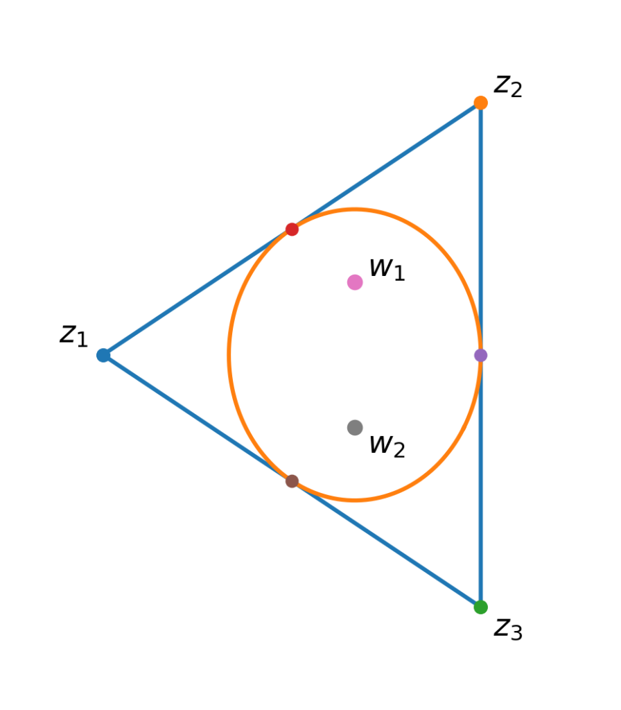
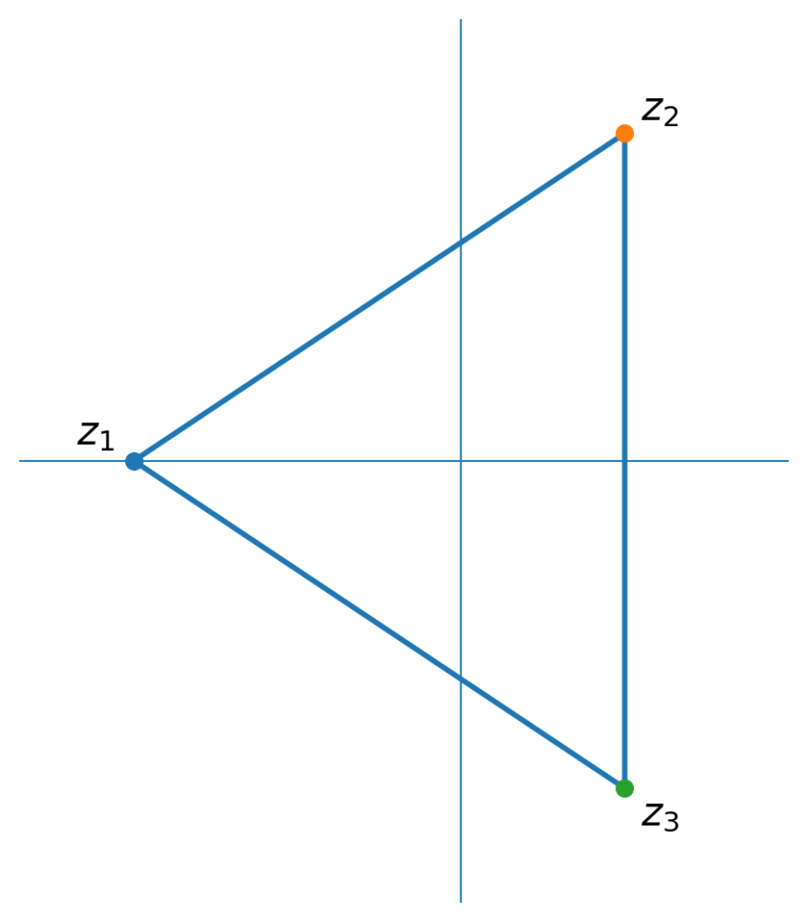
    Three complex roots z1, z2, and z3 plotted as points in the complex plane and joined to form a triangle.
    Figure 1. Three noncollinear roots z₁, z₂, and z₃ of a cubic polynomial determine a triangle in the complex plane.

    What does the derivative know about the triangle?

    There is already a classical theorem that gives us some information. The Gauss–Lucas theorem states that the zeros of the derivative of a polynomial lie in the convex hull of the zeros of the polynomial.

    For our cubic, the convex hull of the three roots is simply the triangle with vertices z1, z2, z3. Therefore the two zeros of p′ must lie inside this triangle.

    That is already an interesting connection between differentiation and geometry. But for a cubic, something much stronger is true.

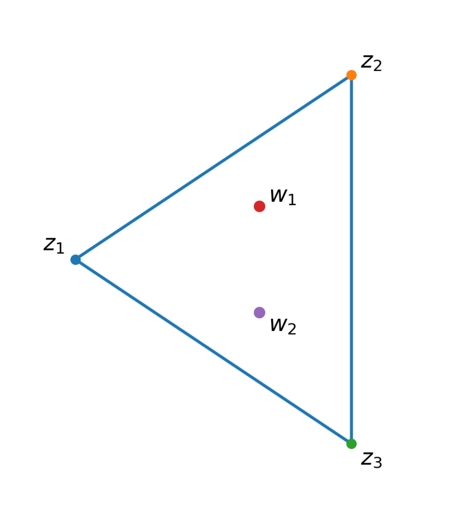
    Triangle formed by three complex roots z1, z2, and z3, with the two derivative zeros w1 and w2 shown inside the triangle.
    Figure 2. By the Gauss–Lucas theorem, the two zeros w₁ and w₂ of the derivative lie inside the triangle determined by the three roots of the cubic.

    Marden’s theorem

    Recall the Steiner inellipse of a triangle: the unique ellipse tangent to the three sides at their midpoints.

    We discussed this ellipse and an area characterization of it in The Steiner Inellipse and a Surprising Area Characterization .

    Marden’s theorem reveals a completely different way in which the same ellipse appears.

    Marden’s Theorem. Let

    p(z) = (z−z1) (z−z2) (z−z3),

    where the three roots are noncollinear. Then the two zeros of p′(z) are exactly the two foci of the Steiner inellipse of the triangle whose vertices are z1, z2, z3.

    This is much stronger than Gauss–Lucas. Gauss–Lucas tells us that the critical points are somewhere inside the triangle. Marden’s theorem identifies their exact geometric meaning.

    The derivative of the cubic has found the foci of an ellipse determined by the roots of the original polynomial.

    Triangle formed by three complex roots with its Steiner inellipse tangent at the side midpoints. The two zeros of the derivative are marked at the two foci of the ellipse.
    Figure 3. Marden’s theorem: the two zeros w₁ and w₂ of the derivative are exactly the foci of the Steiner inellipse of the triangle formed by z₁, z₂, and z₃.

    A concrete example

    Let us see the theorem in action. Choose the three roots

    z1=−2, z2=1+2i, z3=1−2i.

    The corresponding cubic is

    p(z) = (z+2) (z−1−2i) (z−1+2i).

    Multiplying the conjugate factors first gives

    (z−1−2i) (z−1+2i) = z2 −2z +5.

    Hence

    p(z) = (z+2) ( z2 −2z +5 ) = z3 +z +10.

    Now differentiate:

    p′(z) = 3z2 +1.

    The critical points satisfy

    3z2 +1 =0,

    so

    z = ± i 3 .

    Marden’s theorem now tells us something geometric that would be very difficult to guess merely by looking at the polynomial:

    The two foci of the Steiner inellipse are

    i3 and − i3.
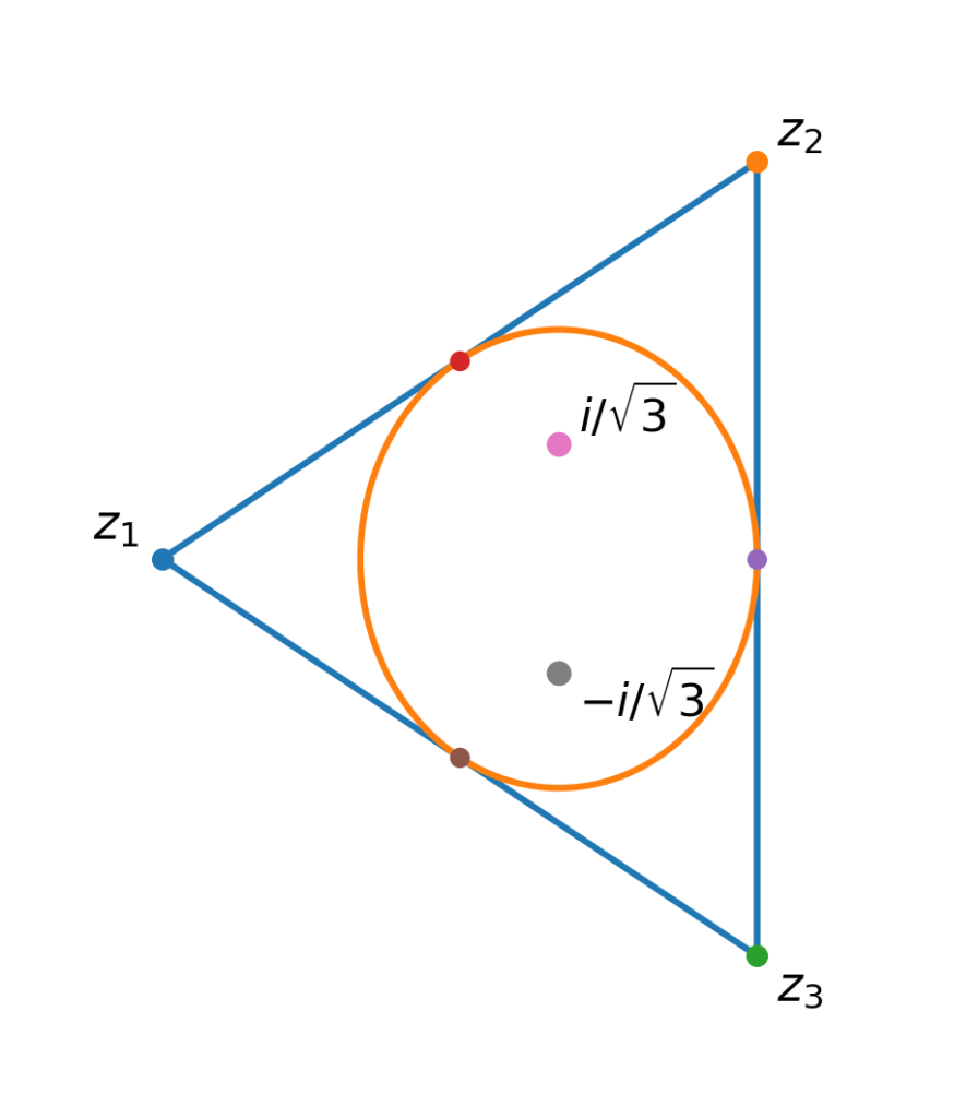
    Triangle with complex roots negative 2, 1 plus 2i, and 1 minus 2i, together with its Steiner inellipse. The two foci are located at i over square root of 3 and negative i over square root of 3.
    Figure 4. For p(z) = z³ + z + 10, the roots form the displayed triangle, while the zeros ±i/√3 of p′(z) are exactly the foci of its Steiner inellipse.

    Why is this so surprising?

    The derivative is usually introduced as an analytic object: it measures instantaneous rate of change, gives the slope of a tangent line, and locates critical points.

    Here it is doing something that looks completely different.

    Start with three complex numbers. Use them as the roots of a cubic. Differentiate the polynomial. Solve one quadratic equation. The two answers are not merely points somewhere inside the triangle—they are the two foci of a distinguished ellipse.

    In symbols, the chain of ideas is

    three roots → triangle → differentiate → two critical points → two foci.

    The same Steiner inellipse therefore admits two very different descriptions.

    In our earlier article, it appeared from an area condition: a point lies on the ellipse precisely when three corner triangles have total area equal to half the area of the original triangle.

    Here the ellipse appears from differentiation: its two foci are the zeros of the derivative of the cubic whose roots are the vertices of the triangle.

    This is a beautiful example of a recurring theme in mathematics: algebra, calculus, and geometry can encode the same object in completely different ways.

    References and further reading

    1. D. Kalman, “An Elementary Proof of Marden’s Theorem” , The American Mathematical Monthly, Vol. 115, No. 4 (2008), pp. 330–338.
    2. A. Eydelzon, “On a New Property of the Steiner Inellipse” , The American Mathematical Monthly, Vol. 127, No. 10 (2020), pp. 933–935.
  • Steiner Inellipse: A Surprising Area Characterization

    Given a triangle, there are many ellipses that can be drawn inside it. Among them, one has a particularly beautiful and distinguished place in geometry: the Steiner inellipse.

    What is the Steiner inellipse?

    Let ABC be any triangle. The Steiner inellipse is the unique ellipse contained in the triangle that is tangent to the three sides at their midpoints.

    Thus, if D, E, and F are the midpoints of BC, CA, and AB, respectively, the Steiner inellipse passes through all three points and is tangent to the corresponding sides there.

    Its center is the centroid G of the triangle—the point where the three medians intersect.

    The Steiner inellipse also has an extremal property: among all ellipses contained in a given triangle, it has the largest possible area.

    Why does the Steiner inellipse naturally appear?

    One way to understand the Steiner inellipse is through affine geometry. Every triangle can be obtained from an equilateral triangle by an invertible affine transformation.

    For an equilateral triangle, the Steiner inellipse is simply its incircle. The incircle touches the three sides at their midpoints and is centered at the common centroid, incenter, and circumcenter.

    Under an affine transformation, a circle generally becomes an ellipse, midpoints remain midpoints, and tangency is preserved. Therefore the incircle of an equilateral triangle is transformed into an ellipse tangent to the three sides of the new triangle at their midpoints. That ellipse is precisely the Steiner inellipse.

    So the Steiner inellipse may be viewed as the affine image of the incircle of an equilateral triangle.

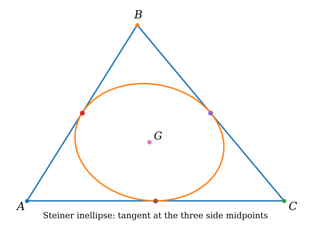
    Triangle ABC containing the Steiner inellipse, tangent to each side at its midpoint and centered at centroid G.
    Figure 1. The Steiner inellipse of triangle ABC.
    It is the unique ellipse tangent to the three sides at their midpoints,
    and its center is the centroid G.

    A different way to recognize the same ellipse

    The definition above characterizes the Steiner inellipse by tangency: it touches the sides of the triangle at three special points.

    But there is another, rather unexpected way to detect whether a point lies on this ellipse—one that does not initially mention an ellipse, tangency, or even distances.

    It uses only parallel lines and areas.

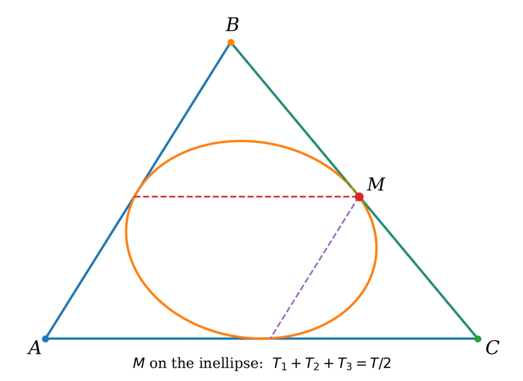
    Choose an arbitrary point M inside triangle ABC. Through M, draw three lines, each parallel to one side of the triangle.

    These three lines cut off three smaller triangles at the vertices A, B, and C. Let their areas be

    T1 , T2 , T3 .

    Let T denote the area of the original triangle.

    Now ask a simple question:

    For which points M is the sum of the three corner areas exactly one-half of the area of the original triangle?

    T1 + T2 + T3 = T2 ?

    At first glance, there is no obvious reason that the answer should involve an ellipse at all.

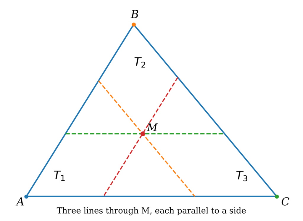
    Triangle ABC with an interior point M and three lines through M parallel to the sides, forming three corner triangles labeled T₁, T₂, and T₃.
    Figure 2. Through an arbitrary interior point M,
    draw three lines parallel to the sides of triangle ABC.
    The three corner triangles have areas T₁, T₂, and T₃.

    The surprising answer

    The answer is remarkably simple: the points satisfying this area condition are exactly the points on the Steiner inellipse.

    Theorem. Let ABC be a triangle with area T , and let M be a point in its interior. Through M, draw three lines parallel to the sides of the triangle, cutting off three corner triangles with areas T1 , T2 , and T3 . Then

    M ∈ Steiner inellipse ⇔ T1 + T2 + T3 = T 2 .

    In other words, a point M lies on the Steiner inellipse if and only if the three corner triangles together have exactly half the area of the original triangle.

    This is unexpected because the construction itself contains no ellipse. We choose a point, draw three parallel lines, and measure three areas. Yet the condition that their sum equals one-half of the total area traces out precisely the Steiner inellipse.

    Why should this be an ellipse?

    The key is affine geometry. An invertible affine transformation sends triangles to triangles, preserves parallelism and ratios of areas, and sends ellipses to ellipses.

    We can therefore transform our original triangle into an equilateral triangle without changing the essential area condition. In an equilateral triangle, the Steiner inellipse becomes something much more familiar: the incircle.

    So it is enough to determine which points satisfy the area condition in the equilateral case.

    Triangle ABC with its Steiner inellipse and a point M on the ellipse. Three lines through M parallel to the sides illustrate the three corner triangles whose total area is half the area of triangle ABC.
    Figure 3. A point M on the Steiner inellipse.
    For this point, the three corner areas satisfy T₁ + T₂ + T₃ = T/2.

    The equilateral case

    Consider the equilateral triangle with vertices

    A=(−1,0), B=(0,3), C=(1,0).

    The base has length 2 and the height is 3 , so the area of the triangle is

    T = 2·3 2 = 3.

    Let M=(a,b) be an interior point. The three lines through M parallel to the sides cut off three smaller triangles. Because each corner triangle is similar to the original equilateral triangle, their areas can be written in terms of a and b.

    A direct calculation gives

    T1 = 34 ( 1 +a − b3 ) 2 , T2 = 34 ( 1 −a − b3 ) 2 ,

    and

    T3 = b2 3 .

    Now impose our area condition:

    T1 + T2 + T3 = T2 = 32.

    Substituting the three expressions above and simplifying gives

    a2 + b2 − 2b 3 = 0.

    Completing the square transforms this into

    a2 + ( b − 13 ) 2 = 13.

    But this is the equation of the circle centered at

    ( 0, 13 )

    with radius 13. This is precisely the incircle of our equilateral triangle.

    Therefore, in the equilateral case, the points satisfying

    T1 + T2 + T3 = T2

    are exactly the points on the incircle.

    Equilateral triangles often turn geometric questions into especially elegant problems. For another example, see Equilateral Triangle Maximum Area .

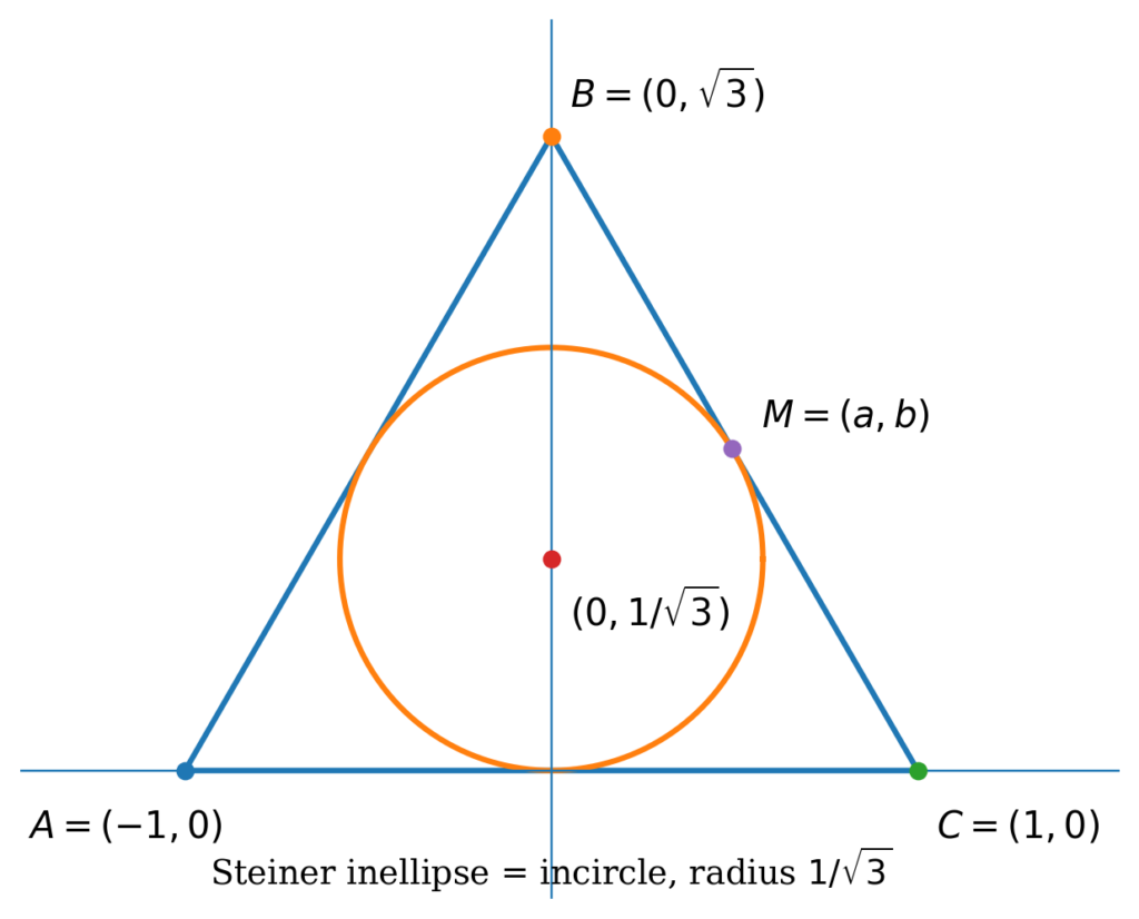
    Equilateral triangle with vertices A, B, and C and its incircle. The circle is centered at (0, 1/√3), has radius 1/√3, and contains the point M = (a,b).
    Figure 4. In the equilateral case, the Steiner inellipse is the incircle. The area condition produces a circle centered at (0, 1/√3) with radius 1/√3.

    Returning to the original triangle

    We have proved that, for an equilateral triangle, the condition

    T1 + T2 + T3 = T2

    describes exactly the incircle.

    Now apply the inverse affine transformation that carries the equilateral triangle back to the original triangle. Parallel lines remain parallel, and all areas are multiplied by the same factor, so the area condition is preserved. The incircle is transformed into the Steiner inellipse.

    Therefore, for any triangle, a point M satisfies the area condition if and only if M lies on the Steiner inellipse.

    A related area identity

    There is another elegant relation involving the same three corner triangles. Unlike the characterization above, this identity holds for every interior point M, not only for points on the Steiner inellipse.

    Since each corner triangle is similar to the original triangle, the ratio of corresponding side lengths is the square root of the ratio of the corresponding areas. The three relevant length ratios add to 1, which gives

    T1 + T2 + T3 = T .

    The contrast between the two identities is worth noticing.

    For every interior point M,

    T1 + T2 + T3 = T.

    But without the square roots,

    T1 + T2 + T3 = T2

    holds precisely when M lies on the Steiner inellipse. Thus the same three corner areas give both a universal identity and a geometric characterization of a special ellipse.

    There is another remarkable way in which the Steiner inellipse appears. If the vertices of the triangle are regarded as the three complex roots of a cubic polynomial, the zeros of its derivative are exactly the two foci of the Steiner inellipse. See Marden’s Theorem: How the Derivative of a Cubic Finds an Ellipse .

    References and further reading

    1. A. Eydelzon, “On a New Property of the Steiner Inellipse” , The American Mathematical Monthly, Vol. 127, No. 10 (2020), pp. 933–935.
    2. NCS/MAA Team Contest, Thirteenth Annual Contest (2009), Problem 9 , “Square roots of area ratios.”
    3. D. Kalman, “An Elementary Proof of Marden’s Theorem” , The American Mathematical Monthly, Vol. 115, No. 4 (2008), pp. 330–338.

    The first reference contains the area characterization of the Steiner inellipse discussed in this article. The second gives an earlier appearance of the classical square-root area problem. The third provides additional background on the Steiner inellipse and its connection with Marden’s theorem.

    A triangle is a two-dimensional simplex, while a tetrahedron is its three-dimensional counterpart. For a related exploration of simplex geometry, see The Geometry of a Tetrahedron: From Pythagoras to Vector Identities .

  • Is the Brachistochrone Still a Cycloid Underwater?

    One of the most beautiful problems in calculus asks:

    What path allows an object, starting from rest, to travel between two points under gravity in the least possible time?

    The shortest path is a straight line. But the fastest path is not. In the classical brachistochrone problem, the answer is a cycloid.

    But there is an assumption hidden inside this famous result: there is no resistance.

    What happens if the object moves through a fluid? Is the fastest path in water, oil, or another viscous medium still a cycloid?

    The answer is no longer universal. Once resistance is present, the optimal path depends on the law of motion itself.


    1. The Classical Brachistochrone

    Suppose an object starts from rest and moves under gravity without friction. Let y measure vertical distance downward from the starting point.

    Conservation of energy gives

    1 2 m v2 = mgy.

    Therefore

    v = 2gy .

    If s denotes distance measured along the curve, then speed is

    v = ds dt .

    Therefore

    dt = ds v .

    The total travel time is consequently

    T = ∫ ds 2gy .

    For a curve written as y = y(x),

    ds = 1 + dy dx 2 dx.

    Thus

    T = ∫ 1 + dy dx 2 2gy dx.

    Minimizing this integral leads to the cycloid.


    2. The Exact Cycloid

    With y positive downward, the cycloid can be parametrized as

    x(θ) = a ( θ − sin(θ) ),
    y(θ) = a ( 1 − cos(θ) ).

    The constants are determined by the endpoint.

    The cycloid illustrates the central idea behind the brachistochrone. The curve initially descends very steeply. Although this makes the path longer than a straight line, the object gains speed quickly and then uses that speed during the remainder of the trip.


    3. What Changes When There Is Resistance?

    The classical derivation relies on conservation of mechanical energy. With drag, mechanical energy is continually dissipated.

    Consequently, the speed can no longer be determined from height alone. Two objects arriving at the same height along two different paths may have different speeds because they have experienced different histories of drag.

    This destroys the simple relation

    v = 2gy .

    Now the path and the velocity must be determined together.


    4. Linear Drag

    A particularly useful mathematical model assumes that the drag force is proportional to speed:

    FD = bv.

    For a small sphere in the Stokes regime,

    b = 6πμR,

    where μ is the dynamic viscosity and R is the radius of the sphere.

    Let s denote arc length along the unknown path. Since

    v = ds dt ,

    the tangential equation of motion is

    m dv dt = mg dy ds − bv.

    Using

    dv dt = dv ds ds dt = v dv ds,

    we obtain

    mv dv ds = mg dy ds − bv.

    5. What Are We Minimizing?

    The quantity we want to minimize is the total travel time. By definition,

    v = ds dt .

    Solving for the small amount of time required to travel the distance ds gives

    dt = ds v .

    Therefore, for a path of total length S,

    T = ∫ 0 S ds v .

    In words,

    time = distance / speed.

    The important difference from the classical brachistochrone is that, in the presence of drag, the speed v is not determined by height alone. It depends on how the object arrived at its current position.

    Thus the viscous brachistochrone problem is to find a path and its corresponding velocity that satisfy the equation of motion while making the total travel time as small as possible.


    6. Buoyancy

    If the object is immersed in a fluid, buoyancy can also be included. For a body of density ρs in a fluid of density ρf, the effective downward acceleration is

    geff = g ( 1 − ρf ρs ).

    In the equation of motion, g can then be replaced by geff.


    7. Water Does Not Automatically Mean Linear Drag

    There is an important physical qualification. Stokes’ linear drag law applies only in an appropriate low-Reynolds-number regime.

    The Reynolds number is

    Re = ρvL μ .

    At higher Reynolds numbers, a quadratic drag model is often more appropriate:

    FD = 1 2 ρf CD A v2.

    If

    k = 1 2 ρf CD A,

    then the corresponding tangential equation is

    mv dv ds = mg dy ds − kv2.

    So there is no single mathematical object called the underwater brachistochrone. The answer depends on the object, the fluid, and the appropriate drag law.


    8. A Numerical Example

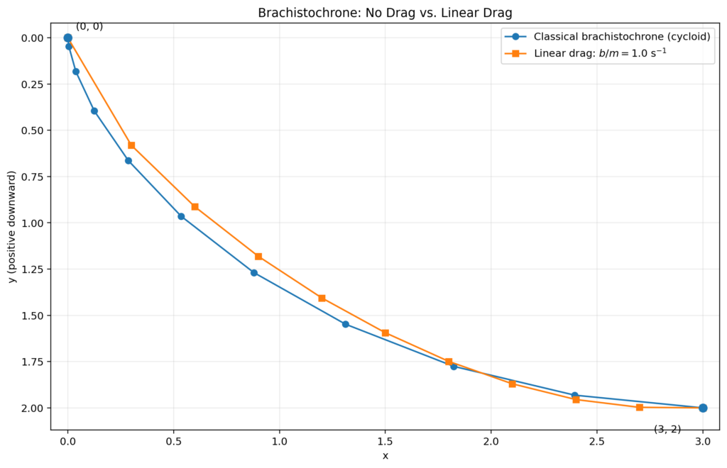
    Let us compare two minimum-time paths having the same endpoints:

    (0,0) and (3,2).

    As before, y is measured downward.

    Case A: No Drag

    For the classical cycloid,

    x = a ( θ − sin(θ) ),
    y = a ( 1 − cos(θ) ).

    The endpoint conditions give approximately

    θf ≈ 3.068777, a ≈ 1.001327.

    Selected points on the exact cycloid are:

    θ x y
    0.00000.00000.0000
    0.30690.00480.0468
    0.61380.03790.1828
    0.92060.12480.3952
    1.22750.28620.6643
    1.53440.53580.9649
    1.84130.87881.2689
    2.14811.31201.5479
    2.45501.82351.7758
    2.76192.39441.9313
    3.06883.00002.0000

    Case B: Linear Drag

    Now keep the same endpoints but introduce linear resistance with

    b m = 1.0 s −1 ,

    and take

    g = 9.81 m s2 .

    This is a mathematical linear-drag example. We do not label it “water” or “oil,” because identifying a real fluid requires checking which drag law is physically appropriate.

    The unknown curve can be approximated numerically by short segments. For each candidate path, the equation of motion is integrated along the path, the travel time is computed, and the intermediate heights are varied to reduce that time.

    Selected points from the numerical minimum-time path are:

    x y
    0.0000.000
    0.3000.581
    0.6000.913
    0.9001.181
    1.2001.406
    1.5001.595
    1.8001.749
    2.1001.870
    2.4001.955
    2.7001.997
    3.0002.000

    9. Something Unexpected Happens

    It is tempting to imagine that adding resistance simply moves the entire brachistochrone to one side of the classical cycloid.

    The numerical example shows that this is not what happens.

    For comparison, evaluating the classical cycloid at the same horizontal positions gives approximately:

    x Linear-drag y Cycloid y
    0.00.0000.000
    0.30.5810.684
    0.60.9131.029
    0.91.1811.285
    1.21.4061.484
    1.51.5951.643
    1.81.7491.767
    2.11.8701.863
    2.41.9551.932
    2.71.9971.978
    3.02.0002.000

    At x = 1.8, the linear-drag path has y approximately 1.749, while the cycloid has y approximately 1.767.

    But at x = 2.1, the linear-drag path has y approximately 1.870, while the cycloid has y approximately 1.863.

    Therefore the two curves cross somewhere between these positions.

    This is a useful warning against relying only on intuition. Resistance does not merely shift the classical cycloid uniformly upward or downward. It changes the optimization problem itself and can change the shape in a more subtle way.


    10. Why Does Drag Change the Answer?

    In the frictionless problem, speed gained early is retained. This makes a steep initial descent extremely valuable.

    With drag, there is a competing effect. Descending early still produces speed, but resistance continually removes energy. Speed acquired early is therefore not as valuable as it is in the frictionless problem.

    The optimal curve must balance:

    • gaining speed quickly by descending,
    • the extra distance caused by that descent, and
    • the continual loss of energy to resistance.

    That competition produces a different minimum-time path.


    11. There Is No Single “Brachistochrone in Water”

    This is perhaps the most important physical lesson.

    Changing the medium can change the viscosity, density, buoyancy, Reynolds number, drag coefficient, and even the mathematical form of the drag law. Changing the size or shape of the moving object can do the same.

    Therefore asking

    “What is the brachistochrone in water?”

    does not completely specify the problem.

    A more precise question is:

    For this object, in this fluid, under this drag law, what path minimizes the travel time?

    12. The Bigger Lesson

    The classical brachistochrone is famous because the answer is unexpectedly beautiful: a cycloid.

    But there is an even broader lesson hiding behind it.

    The fastest path is not determined by geometry alone. It depends on the law of motion.

    With no resistance, the answer is a cycloid. With viscous resistance, the speed remembers the history of the path, and the optimization problem changes. For other drag laws, it changes again.

    So perhaps the more interesting question is not

    “What is the fastest curve?”

    but rather

    “What physical laws make a particular curve the fastest?”
    Classical cycloid and numerical linear-drag brachistochrone from (0, 0) to (3, 2), showing the two optimal paths crossing.
    Classical cycloid and numerical linear-drag brachistochrone from (0, 0) to (3, 2), showing the two optimal paths crossing.

    Another example where the mathematics of motion produces a surprising result is my related-rates problem about a sliding ladder: is it safer to slide or jump?

  • Projectile Motion in 3D: Adding Wind and Air Resistance

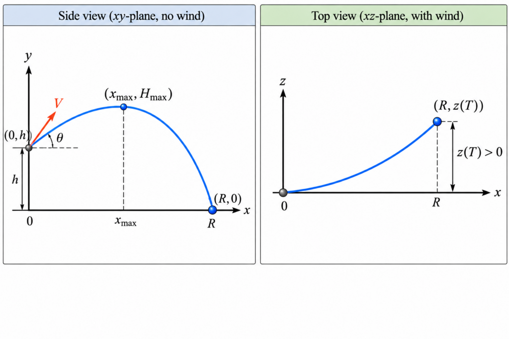
    The standard projectile-motion problem is familiar from calculus and physics: a projectile is launched with initial speed V at an angle θ above the horizontal from an initial height h. Gravity pulls it downward, and we ask two basic questions:

    • How high does the projectile go?
    • How far does it travel before hitting the ground?

    But real projectiles do not necessarily stay in a vertical plane. What happens if we add a horizontal wind blowing from the side? And what happens if we also include air resistance?

    The familiar two-dimensional parabola becomes a genuinely three-dimensional trajectory. With a simple model of air resistance, we can still obtain explicit formulas for almost everything.

    1. Setting Up the Coordinates

    Choose coordinates so that:

    • x is the original horizontal firing direction,
    • y is the vertical direction,
    • z is the sideways horizontal direction.

    The projectile is fired in the vertical xy-plane, so initially there is no velocity in the z-direction.

    The initial position is

    r (0) = ( 0,h,0 ).

    The initial velocity is

    v (0) = ( V⁢cos⁡θ , V⁢sin⁡θ ,0 ).

    2. Adding Wind

    Suppose a horizontal wind has speed W and makes an angle φ with the positive x-direction. Its velocity vector is

    w= ( W⁢cos⁡φ ,0, W⁢sin⁡φ ).

    The component W⁢cos⁡φ pushes along the original firing direction, while W⁢sin⁡φ produces sideways motion.

    3. Air Resistance Must Be Relative to the Air

    If there were no air resistance, a steady wind would have no effect on an ideal point projectile. Wind matters because the projectile interacts with the surrounding air.

    For a simple model, assume that air resistance is proportional to the projectile’s velocity relative to the moving air. If k is the drag constant per unit mass, the acceleration due to air resistance is

    −k ( v − w ).

    Gravity contributes

    ( 0,−g,0 ).

    Therefore the equation of motion is

    r″ = −gj −k ( r′ − w ).

    4. Three Differential Equations

    Writing the vector equation component by component gives

    x″ = −k ( x′ − W⁢cos⁡φ ) y″ = −g −ky′ z″ = −k ( z′ − W⁢sin⁡φ ).

    Although the trajectory is three-dimensional, something very convenient has happened: the three equations can be solved separately.

    5. Solving for the Velocity

    The velocity in the x-direction is

    vx (t) = W⁢cos⁡φ + ( V⁢cos⁡θ − W⁢cos⁡φ ) e−kt.

    The sideways velocity is

    vz (t) = W⁢sin⁡φ ( 1− e−kt ).

    The vertical velocity is

    vy (t) = ( V⁢sin⁡θ + gk ) e−kt − gk.

    Notice the long-term behavior. The horizontal velocity approaches the wind velocity, while the vertical velocity approaches

    −gk.

    In this linear-drag model, this is the terminal vertical velocity.

    6. The 3D Position

    Integrating the velocity components and using the initial position gives

    x (t) = W⁢cos⁡φt + V⁢cos⁡θ − W⁢cos⁡φ k ( 1− e−kt ). y (t) = h − gkt + V⁢sin⁡θ +gk k ( 1− e−kt ). z (t) = W⁢sin⁡φ [ t − 1− e−kt k ].

    These three equations describe the complete trajectory through space. Unlike the usual projectile trajectory, this curve is not a parabola.

    7. When Does the Projectile Reach Its Maximum Height?

    At maximum height the vertical velocity is zero:

    vy ( tmax ) =0.

    Therefore

    ( V⁢sin⁡θ +gk ) e −ktmax = gk.

    Solving for time gives

    tmax = 1k ln⁡ ( 1 + kV⁢sin⁡θ g ).

    8. Maximum Height

    Substituting this time into the vertical position formula and simplifying gives

    Hmax = h + V⁢sin⁡θ k − gk2 ln⁡ ( 1 + kV⁢sin⁡θ g ).

    An interesting consequence is that the horizontal wind does not appear in this formula. In this model, horizontal wind changes where the projectile lands, but it does not change its maximum height.

    9. When Does It Hit the Ground?

    Let T denote the time at which the projectile hits the ground. We find T by setting

    y (T) =0.

    Thus T satisfies

    h − gkT + V⁢sin⁡θ + gk k ( 1− e−kT ) =0.

    Here we encounter an important difference from the standard projectile problem. Without air resistance, finding the flight time requires solving a quadratic equation. With linear air resistance, the unknown T appears both outside and inside an exponential.

    In practice, the positive solution can be found numerically using a calculator, computer, graphing program, or Newton’s method.

    10. Where Does It Land?

    Once the flight time T has been found, the landing point is

    ( x(T) , 0 , z(T) ).

    The downrange distance in the original firing direction is x(T) , while the sideways displacement is z(T) .

    The total horizontal distance between the launch point and landing point is

    R= x(T) 2 + z(T) 2 .

    So in three dimensions, the question “How far does the projectile go?” has more than one possible answer. We can ask for its downrange distance, its sideways drift, or its total horizontal displacement.

    11. How Far Sideways Does the Wind Push It?

    The sideways displacement at landing is

    z (T) = W⁢sin⁡φ [ T − 1− e−kT k ].

    This is zero when the wind blows exactly along the original firing direction. It becomes nonzero when the wind has a crosswind component.

    12. A Consistency Check: Remove Air Resistance

    A good mathematical model should reproduce the familiar result when the new effect is removed. Let the drag coefficient k approach zero. A key limit is

    lim k→0 1− e−kt k =t.

    As air resistance disappears, the vertical motion approaches

    y (t) = h + V⁢sin⁡θt − 12 gt2,

    which is exactly the standard projectile-motion formula.

    The maximum-height formula also approaches

    Hmax → h + V2 sin⁡θ 2 2g .

    Again, this is precisely the familiar result.

    13. From a Parabola to a Space Curve

    The ordinary projectile problem is two-dimensional. Its trajectory is a parabola contained in a vertical plane.

    Adding a crosswind and air resistance changes the geometry completely. The projectile now moves simultaneously forward, vertically, and sideways. Its position is described parametrically by

    r (t) = ( x(t) , y(t) , z(t) ).

    This is a natural example of why parametric vector equations are useful: there is no need to force a three-dimensional trajectory into a single equation involving x, y, and z.

    14. What Makes This Problem Interesting?

    The standard projectile problem is often presented as an application of quadratic functions. But a relatively small change in the physical assumptions leads to much richer mathematics.

    The three-dimensional model combines:

    • vectors and parametric curves,
    • differential equations,
    • exponential functions,
    • optimization,
    • numerical root finding,
    • limits,
    • and mathematical modeling.

    Most importantly, the model separates two questions that look similar but are physically different. Gravity and vertical drag determine when the projectile hits the ground. The wind and horizontal drag then determine where it lands.

    That is the real advantage of moving from the familiar two-dimensional projectile problem to a three-dimensional model: instead of asking only “How far?”, we can ask the more interesting question: Where will it land?

    Worked Example: Where Does the Projectile Land?

    Let us use the formulas above with actual numbers. Suppose a projectile is launched from a height of 10 meters with an initial speed of 40 m/s at an angle of 45° above the horizontal.

    A horizontal wind blows at 10 m/s at an angle of 60° from the original firing direction. Assume a linear drag constant k = 0.10 s−1 and take g = 9.81 m/s2.

    Thus our data are

    h=10 m,   V=40 m/s,   θ=45°, W=10 m/s,   φ=60°,   k=0.10 s −1.

    Step 1: When Does It Reach Maximum Height?

    The time at which the projectile reaches its maximum height is

    tmax = 1k ln⁡ ( 1 + kV ⁢ sin⁡θ g ).

    Substituting the numerical values gives

    tmax = 10.10 ln⁡ ( 1 + ( 0.10 ) ( 40 ) sin⁡ 45° 9.81 ).

    Therefore,

    tmax ≈ 2.533 s.

    The projectile reaches its highest point about 2.53 seconds after launch.

    Step 2: What Is the Maximum Height?

    The maximum height is

    Hmax = h + V ⁢ sin⁡θ k − g k2 ln⁡ ( 1 + kV ⁢ sin⁡θ g ).

    Substitution gives

    Hmax = 10 + 40 sin⁡ 45° 0.10 − 9.81 0.102 ln⁡ ( 1 + ( 0.10 ) ( 40 ) sin⁡ 45° 9.81 ).

    Thus

    Hmax ≈ 44.32 m.

    The projectile rises to approximately 44.32 meters above the ground.

    Step 3: When Does It Hit the Ground?

    The projectile hits the ground when y ( T ) =0 . For our values, this means solving

    10 − 9.810.10T + 40 sin⁡ 45° + 9.810.10 0.10 ( 1 − e −0.10T ) =0.

    Unlike the standard projectile problem, this is not a quadratic equation. The unknown T appears both by itself and in an exponential. Solving the equation numerically gives

    T ≈ 5.698 s.

    So the projectile is in the air for approximately 5.70 seconds.

    Step 4: How Far Downrange Does It Travel?

    The horizontal x-coordinate at landing is

    x ( T ) = W ⁢ cos⁡φ ⁢T + V ⁢ cos⁡θ − W ⁢ cos⁡φ k ( 1 − e −kT ).

    Substituting T≈5.698 gives

    x ( T ) ≈ 129.62 m.

    Thus the projectile travels approximately 129.62 meters downrange.

    Step 5: How Far Sideways Does the Wind Push It?

    The sideways coordinate at landing is

    z ( T ) = W ⁢ sin⁡φ [ T − 1 − e −kT k ].

    Substituting the numerical values gives

    z ( T ) = 10 sin⁡ 60° [ 5.698 − 1 − e − ( 0.10 ) ( 5.698 ) 0.10 ].

    Therefore,

    z ( T ) ≈ 11.73 m.

    The wind has pushed the projectile approximately 11.73 meters sideways from the original vertical firing plane.

    Step 6: Where Does It Land?

    We now know both horizontal coordinates. Therefore the landing point is approximately

    P = ( 129.62 , 0 , 11.73 ) m.

    In other words, the projectile lands approximately 129.62 meters downrange and 11.73 meters sideways from the original vertical firing plane.

    Step 7: Total Horizontal Displacement

    The straight-line horizontal distance from the point directly below the launch position to the landing point is

    R = x ( T ) 2 + z ( T ) 2 .

    Therefore,

    R = 129.622 + 11.732 ≈ 130.15 m.

    The Answer

    For this example, the projectile reaches a maximum height of approximately 44.32 m and stays in the air for approximately 5.70 s.

    It lands approximately 129.62 m downrange and 11.73 m sideways from the original vertical firing plane. Thus its landing point is

    ( 129.62 , 0 , 11.73 ) m.

    The total horizontal displacement from the point directly below the launch position is approximately 130.15 m. The sideways displacement shows exactly how the wind changes the familiar two-dimensional projectile problem into a three-dimensional one.


    For another example of how calculus can reveal something unexpected in a real-world motion problem, see Sliding Ladder: Is It Better to Slide or Jump?.

    Projectile motion and planetary motion are both governed by Newton’s laws. Near Earth’s surface, gravity is approximately constant, while planetary orbits require the inverse-square law of gravitation. Explore this connection in Kepler’s Laws: How Calculus Explains Planetary Motion .

  • A Sliding Ladder: Is It Better to Slide or Jump?

    The sliding-ladder problem is one of the most familiar examples of related rates in calculus.

    A ladder leans against a vertical wall. The bottom begins to slide away from the wall, while the top slides downward.

    Usually the textbook asks:

    How fast is the top of the ladder moving?

    But there is a more interesting question:

    If you were on the ladder when it started to slide, what would the mathematics predict as the ladder approached the floor?

    The answer is surprising.

    The Geometry

    Suppose the ladder has fixed length L. Let x be the distance from the bottom of the ladder to the wall, and let y be the height of the top of the ladder above the floor.

    Because the ladder, wall, and floor form a right triangle,

    x2 + y2 = L2 .

    As the ladder slides, both x and y change with time. Differentiate with respect to t:

    2x dx dt + 2y dy dt = 0 .

    Dividing by 2 gives

    x dx dt + y dy dt = 0 .

    Therefore,

    dy dt = − xy dx dt .

    This is the standard related-rates formula for a sliding ladder.

    Suppose the Bottom Moves at Constant Speed

    Assume that the bottom of the ladder moves away from the wall at a constant speed v:

    dx dt = v , v>0 .

    Then

    dy dt = − v xy .

    Since

    x = L2 − y2 ,

    we can also write

    dy dt = − v L2 − y2 y .

    The minus sign tells us that the top of the ladder is moving downward.

    What Happens Near the Floor?

    As the top of the ladder approaches the floor,

    y → 0+ , x → L .

    Therefore,

    xy → ∞ ,

    and consequently

    dy dt → −∞ .

    According to this model, the top of the ladder moves downward faster and faster, and its vertical speed becomes arbitrarily large as it approaches the floor.

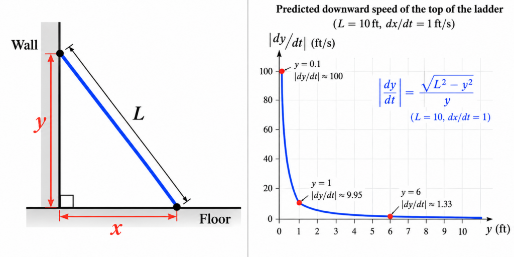
    A Numerical Example

    Suppose the ladder is 10 feet long and its bottom slides away from the wall at

    dx dt = 1 ft/s .

    When the top is 6 feet above the floor,

    x = 100−36 = 8 .

    Thus,

    dy dt = − 86 = − 43 ft/s .

    Nothing dramatic yet. But when the top is only 1 foot above the floor,

    x = 99 ,

    so

    dy dt = −99 ≈ −9.95 ft/s .

    When the top is only 0.1 foot above the floor,

    dy dt = − 99.99 0.1 ≈ −100 ft/s .

    The closer the top gets to the floor, the larger the predicted downward speed becomes.

    What About dy/dx?

    There is another way to see where this strange behavior comes from. Differentiate

    x2 + y2 = L2

    with respect to x. We obtain

    2x + 2y dy dx = 0 ,

    and therefore

    dy dx = − xy .

    As the ladder approaches the floor,

    dy dx → −∞ .

    Geometrically, this makes sense. The point (x,y) moves along the quarter-circle

    x2 + y2 = L2 ,

    which has a vertical tangent at (L,0) .

    But there is an important distinction: dy/dx is not a velocity.

    The connection with velocity is

    dy dt = dy dx dx dt .

    If the horizontal speed remains positive and constant while dy dx becomes unbounded, then the predicted vertical velocity becomes unbounded as well.

    So Is It Better to Slide or Jump?

    At first sight, the mathematics seems to give a disturbing answer. If you remain with the ladder, the simple model predicts that the downward speed can become enormous near the floor.

    Does that mean you should jump?

    Not so fast.

    The calculation has actually revealed something more interesting: the mathematical model has become physically unrealistic.

    We assumed that the bottom of the ladder continues moving horizontally at a constant speed all the way until the ladder becomes horizontal. A real ladder cannot behave this way.

    A real ladder has mass and rotational inertia. There is friction between the ladder and the floor and between the ladder and the wall. The ladder may lose contact with the wall. A person standing on it changes the center of mass and the forces acting on the system.

    Most importantly, a real physical system cannot produce the infinite vertical velocity predicted by this simplified model.

    So the infinity does not tell us that a real person will hit the floor at infinite speed.

    It tells us that one of our assumptions must fail before that happens.

    Calculus as a Warning About a Model

    This is what makes the sliding-ladder problem more interesting than the usual textbook exercise.

    Related rates correctly tells us that

    dy dt = − xy dx dt .

    Under the additional assumption that the horizontal speed stays constant, it follows that

    | dy dt | → ∞ .

    The calculus is not wrong. The assumption is unrealistic.

    When a correct calculation produces a physically impossible result, the mathematics may be telling us where our model stops being valid.

    The humble sliding-ladder problem is therefore not just an exercise in implicit differentiation. It is also a lesson about the difference between mathematics and the physical world.


    Related: Another example of mathematics revealing the limitations of a model is Population Growth: From Exponential Growth to the Logistic Equation .


    For another example of how calculus models motion in the real world, see Projectile Motion in 3D: Adding Wind and Air Resistance, where the standard projectile problem is extended to include wind and air resistance.

    Another classical motion problem with a surprising answer is the brachistochrone problem. The fastest path is a cycloid when there is no resistance—but what happens when fluid resistance is added?

    Calculus describes many kinds of motion, from mechanical systems on Earth to planets orbiting the Sun. For a fascinating application of derivatives, geometry, and Newton’s laws, read Kepler’s Laws: How Calculus Explains Planetary Motion .

  • Can a Function Be Continuous Everywhere but Differentiable Nowhere?

    A basic theorem from calculus says that every differentiable function is continuous. But what about the converse?

    If a function is continuous everywhere, must it be differentiable somewhere?

    It seems reasonable. A continuous graph has no jumps or breaks, and we might expect that if we zoom in far enough, at least some part of the graph should begin to look like a straight line.

    Surprisingly, this intuition is completely wrong.

    There are functions that are continuous at every point and yet differentiable at no point.

    Continuous Does Not Mean Smooth

    We learn early in calculus that

    differentiable⟹continuous.

    The reverse implication is false. Continuity only says that nearby inputs give nearby outputs. It does not say that the graph must have a well-defined tangent line.

    A corner such as the one in the graph of f(x)=|x| already shows that a continuous function can fail to be differentiable at a point.

    But that raises a much more surprising question:

    Can a continuous function have a corner-like failure of smoothness everywhere?

    Weierstrass’s Remarkable Example

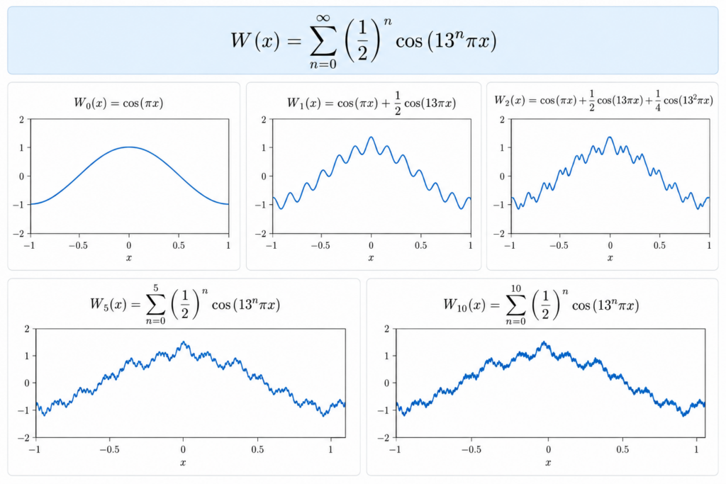
    A famous example is the Weierstrass function, constructed from an infinite sum of cosine waves:

    W(x)=∑n=0∞ancos⁡(bnπx).

    Here 0<a<1 and b is chosen sufficiently large.

    For a concrete example, take

    a=12,b=13.

    Then

    W(x)=∑n=0∞12ncos⁡(13nπx).

    What Is Happening?

    Look carefully at the two competing parts of each term.

    The amplitude is

    an.

    Because 0<a<1, these amplitudes become smaller and smaller.

    But the frequency is controlled by

    bn,

    which becomes larger and larger.

    So every new term adds a smaller wave—but a wave that oscillates much more rapidly than the waves before it.

    Watch the Roughness Appear

    Instead of looking immediately at the infinite sum, consider its partial sums

    WN(x)=∑n=0Nancos⁡(bnπx).

    The first term is just a smooth cosine curve. Adding more terms creates smaller and faster oscillations. The graph becomes increasingly rough.

    Every finite partial sum is still perfectly smooth. The strange behavior appears only in the limit as infinitely many increasingly rapid oscillations are added.

    Why Is the Function Continuous?

    The continuity is actually the easier part. Since

    |ancos⁡(bnπx)|≤an,

    and the geometric series

    ∑n=0∞an=11−a

    converges, the Weierstrass series converges uniformly. Each partial sum is continuous, and a uniform limit of continuous functions is continuous.

    Thus W(x) is continuous everywhere.

    So Why Is It Not Differentiable?

    Here is the intuition.

    At any fixed scale, the graph may appear almost smooth. But when we zoom in, terms with higher frequencies become visible. Zoom in again, and still higher-frequency terms reveal another layer of oscillation.

    There is no scale at which the graph finally settles down into a straight line.

    A derivative would require the difference quotient

    W(x+h)−W(x)h

    to approach a single finite value as h→0. For suitable choices of a and b, the increasingly rapid oscillations prevent this from happening at every point.

    A rigorous proof of nowhere differentiability requires more work, but the mechanism is visible directly in the construction: decreasing amplitudes preserve continuity while rapidly increasing frequencies destroy local smoothness.

    A Change in Mathematical Intuition

    Examples like the Weierstrass function were historically important because they challenged the idea that a continuous curve should be smooth except perhaps at a few exceptional points.

    Continuity turns out to permit behavior far more complicated than our geometric intuition initially suggests.

    A function can have no jumps, no breaks, and no discontinuities anywhere—and still have no tangent line anywhere.

    The Main Surprise

    The Weierstrass function separates two ideas that can look almost identical when we first learn calculus:

    continuity and smoothness are not the same thing.

    Even more remarkably, the failure of smoothness does not have to occur at a few isolated points. It can occur at every single point.


    Continue exploring: Continuous functions can behave strangely in other ways too. Can a Curve Fill a Square? The Mathematics of Space-Filling Curves