The Gaussian Integral and Beyond: From e^(-x²) to a Family of Integrals

Some integrals are easy to write down but surprisingly difficult to evaluate. One of the most famous examples is

$${\int }_{-\infty }^{\infty }{e}^{-x^2}dx.$$

The function $e^{-x^2}$ has no elementary antiderivative. Yet the improper integral has the remarkably simple value

$${\int }_{-\infty }^{\infty }{e}^{-x^2}dx=\sqrt{\pi }.$$

Even more interesting is the method used to obtain this result. By turning a one-dimensional integral into a two-dimensional one, we can exploit geometry. Once we understand that idea, it leads naturally to integrals involving $e^{-x^4}$, $e^{-x^p}$, and even integrals in which the Gaussian is multiplied by a sine or cosine.

Example 1: The Gaussian integral

Let

$$I={\int }_0^{\infty }{e}^{-x^2}dx.$$

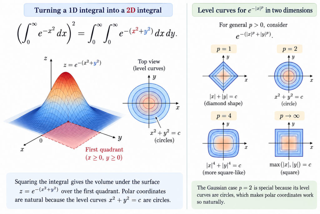
Instead of trying to find an antiderivative, square the integral:

$$I^2=\left({\int }_0^{\infty }{e}^{-x^2}dx\right)\left({\int }_0^{\infty }{e}^{-y^2}dy\right).$$

Thus,

$$I^2={\int }_0^{\infty }{\int }_0^{\infty }{e}^{-(x^2+y^2)}dxdy.$$

Now something important has happened. The expression

$$x^2+y^2$$

suggests polar coordinates. In the first quadrant,

$$x=r\cos (\theta ),y=r\sin (\theta ).$$

Here

$$0\le r<\infty ,0\le \theta \le \frac{\pi }{2}.$$

Since

$$dxdy=rdrd\theta ,$$

we obtain

$$I^2={\int }_0^{\frac{\pi }{2}}{\int }_0^{\infty }{e}^{-r^2}rdrd\theta .$$

The radial integral is elementary:

$${\int }_0^{\infty }{e}^{-r^2}rdr=\frac{1}{2}.$$

Therefore,

$$I^2=\frac{\pi }{2}·\frac{1}{2}=\frac{\pi }{4},$$

and hence

$${\int }_0^{\infty }{e}^{-x^2}dx=\frac{\sqrt{\pi }}{2}.$$

By symmetry,

$${\int }_{-\infty }^{\infty }{e}^{-x^2}dx=\sqrt{\pi }.$$

The essential idea was not integration by parts or an ingenious substitution. It was to increase the dimension.

Example 2: Changing the scale

Consider

$${\int }_0^{\infty }{e}^{-a{x}^2}dx,a>0.$$

Let

$$u=\sqrt{a}x.$$

Then

$$dx=\frac{du}{\sqrt{a}},$$

so

$${\int }_0^{\infty }{e}^{-a{x}^2}dx=\frac{1}{\sqrt{a}}{\int }_0^{\infty }{e}^{-u^2}du=\frac{\sqrt{\pi }}{2\sqrt{a}}.$$

One geometric calculation has already produced an entire family of integrals.

Example 3: An integral involving $e^{-x^4}$

First consider

$${\int }_0^{\infty }{x}^3{e}^{-x^4}dx.$$

The substitution $u=x^4$ works immediately because

$$du=4x^{3}dx.$$

Hence,

$${\int }_0^{\infty }{x}^3{e}^{-x^4}dx=\frac{1}{4}{\int }_0^{\infty }{e}^{-u}du=\frac{1}{4}.$$

Now remove the factor $x^3$.

Example 4: What about $e^{-x^4}$ itself?

Consider

$$J={\int }_0^{\infty }{e}^{-x^4}dx.$$

Let $u=x^4$. Then

$$dx=\frac{1}{4}{u}^{-\frac{3}{4}}du,$$

and therefore

$$J=\frac{1}{4}{\int }_0^{\infty }{u}^{-\frac{3}{4}}{e}^{-u}du.$$

This integral is not elementary, but it is a standard special function. The Gamma function is defined, for $s>0$, by

$$\Gamma (s)={\int }_0^{\infty }{u}^{s-1}{e}^{-u}du.$$

Therefore,

$${\int }_0^{\infty }{e}^{-x^4}dx=\frac{1}{4}\Gamma \left(\frac{1}{4}\right).$$

The Gaussian was already hiding the Gamma function

Apply the same substitution to the Gaussian integral. With $u=x^2$,

$${\int }_0^{\infty }{e}^{-x^2}dx=\frac{1}{2}\Gamma \left(\frac{1}{2}\right).$$

But our two-dimensional calculation showed that the same integral equals $\frac{\sqrt{\pi }}{2}$. Consequently,

$$\Gamma \left(\frac{1}{2}\right)=\sqrt{\pi }.$$

From $e^{-x^2}$ to $e^{-x^p}$

Now consider the general integral

$$I_p={\int }_0^{\infty }{e}^{-x^p}dx,p>0.$$

Set $u=x^p$. Then

$$dx=\frac{1}{p}{u}^{\frac{1}{p}-1}du.$$

Therefore,

$$I_p=\frac{1}{p}{\int }_0^{\infty }{u}^{\frac{1}{p}-1}{e}^{-u}du.$$

By the definition of the Gamma function,

$${\int }_0^{\infty }{e}^{-x^p}dx=\frac{1}{p}\Gamma \left(\frac{1}{p}\right).$$

Using the identity $\Gamma (s+1)=s\Gamma (s)$, we can also write

$${\int }_0^{\infty }{e}^{-x^p}dx=\Gamma \left(1+\frac{1}{p}\right).$$

For example,

$$\begin{array}{l}{\displaystyle {\int }_0^{\infty }{e}^{-x}dx=1,}\\ {\displaystyle {\int }_0^{\infty }{e}^{-x^2}dx=\frac{\sqrt{\pi }}{2},}\\ {\displaystyle {\int }_0^{\infty }{e}^{-x^3}dx=\frac{1}{3}\Gamma \left(\frac{1}{3}\right),}\\ {\displaystyle {\int }_0^{\infty }{e}^{-x^4}dx=\frac{1}{4}\Gamma \left(\frac{1}{4}\right).}\end{array}$$

An even larger family

We can include a power of $x$. Consider

$${\int }_0^{\infty }{x}^q{e}^{-x^p}dx,$$

where $p>0$ and $q>-1$. Again let $u=x^p$. The same substitution gives

$${\int }_0^{\infty }{x}^q{e}^{-x^p}dx=\frac{1}{p}\Gamma \left(\frac{q+1}{p}\right).$$

For example,

$${\int }_0^{\infty }x{e}^{-x^4}dx=\frac{1}{4}\Gamma \left(\frac{1}{2}\right)=\frac{\sqrt{\pi }}{4},$$

while

$${\int }_0^{\infty }{x}^3{e}^{-x^4}dx=\frac{1}{4}\Gamma (1)=\frac{1}{4}.$$

Thus three very similar-looking integrals can have rather different-looking answers:

$$\begin{array}{l}{\displaystyle {\int }_0^{\infty }{e}^{-x^4}dx=\frac{1}{4}\Gamma \left(\frac{1}{4}\right),}\\ {\displaystyle {\int }_0^{\infty }x{e}^{-x^4}dx=\frac{\sqrt{\pi }}{4},}\\ {\displaystyle {\int }_0^{\infty }{x}^3{e}^{-x^4}dx=\frac{1}{4}.}\end{array}$$

Why did circles appear?

There is a geometric reason the Gaussian calculation worked so beautifully. When we squared the Gaussian integral, the exponent became

$$x^2+y^2.$$

The level curves

$$x^2+y^2=c$$

are circles. Polar coordinates are therefore perfectly adapted to the problem.

If instead we square ${\int }_0^{\infty }{e}^{-x^4}dx$, we obtain

$${\int }_0^{\infty }{\int }_0^{\infty }{e}^{-(x^4+y^4)}dxdy.$$

The corresponding level curves are

$$x^4+y^4=c.$$

They are not circles. More generally, $e^{-x^p}$ is naturally connected with regions of the form

$${\left|x\right|}^p+{\left|y\right|}^p\le r^p.$$

For $p=2$, these are ordinary disks. For larger values of $p$, their boundaries become increasingly square-like. The Gaussian is the particularly beautiful case in which the geometry becomes ordinary Euclidean geometry.

A surprising turn: add a cosine

Consider

$$C(b)={\int }_0^{\infty }{e}^{-x^2}\cos (bx)dx.$$

The answer is

$$C(b)=\frac{\sqrt{\pi }}{2}{e}^{-\frac{b^2}{4}}.$$

This is remarkable: multiplying a Gaussian by an oscillating cosine produces another Gaussian, now as a function of the parameter $b$.

Here is a calculus derivation. Differentiate with respect to $b$:

$$C^{\prime }(b)=-{\int }_0^{\infty }x{e}^{-x^2}\sin (bx)dx.$$

Since

$$x{e}^{-x^2}=-\frac{1}{2}\frac{d}{dx}(e^{-x^2}),$$

integration by parts gives

$$C^{\prime }(b)=-\frac{b}{2}C(b).$$

Therefore,

$$\frac{C^{\prime }(b)}{C(b)}=-\frac{b}{2}.$$

Integrating gives

$$C(b)=A{e}^{-\frac{b^2}{4}}.$$

At $b=0$,

$$C(0)={\int }_0^{\infty }{e}^{-x^2}dx=\frac{\sqrt{\pi }}{2}.$$

Thus,

$${\int }_0^{\infty }{e}^{-x^2}\cos (bx)dx=\frac{\sqrt{\pi }}{2}{e}^{-\frac{b^2}{4}}.$$

For example, taking $b=2$ gives

$${\int }_0^{\infty }{e}^{-x^2}\cos (2x)dx=\frac{\sqrt{\pi }}{2e}.$$

What happens with sine?

Now consider

$$S(b)={\int }_0^{\infty }{e}^{-x^2}\sin (bx)dx.$$

Unlike the cosine integral, this does not reduce to an elementary expression involving only exponentials and $\pi$. It can be written using a special function called Dawson’s integral,

$$F(z)=e^{-z^2}{\int }_0^z{e}^{t^2}dt.$$

The result is

$${\int }_0^{\infty }{e}^{-x^2}\sin (bx)dx=F\left(\frac{b}{2}\right).$$

The difference between sine and cosine has a simple symmetry explanation. The function

$$e^{-x^2}\cos (bx)$$

is even, while

$$e^{-x^2}\sin (bx)$$

is odd. Therefore, over the entire real line,

$${\int }_{-\infty }^{\infty }{e}^{-x^2}\sin (bx)dx=0,$$

whereas

$${\int }_{-\infty }^{\infty }{e}^{-x^2}\cos (bx)dx=\sqrt{\pi }{e}^{-\frac{b^2}{4}}.$$

One function keeps returning

We started with $e^{-x^2}$. It has no elementary antiderivative, so at first it seems difficult to work with. But instead of disappearing, the Gaussian keeps returning.

Geometry gives

$${\int }_{-\infty }^{\infty }{e}^{-x^2}dx=\sqrt{\pi }.$$

The Gamma function places it inside the larger family

$${\int }_0^{\infty }{e}^{-x^p}dx=\Gamma \left(1+\frac{1}{p}\right).$$

Adding a power of $x$ produces

$${\int }_0^{\infty }{x}^q{e}^{-x^p}dx=\frac{1}{p}\Gamma \left(\frac{q+1}{p}\right).$$

And adding an oscillating cosine gives another Gaussian:

$${\int }_{-\infty }^{\infty }{e}^{-x^2}\cos (bx)dx=\sqrt{\pi }{e}^{-\frac{b^2}{4}}.$$

This last identity is a glimpse of a much deeper fact: under the Fourier transform, the Gaussian essentially transforms into itself.

So a single integral that cannot be evaluated by ordinary antiderivatives opens the door to geometry, the Gamma function, differential equations, generalized $L^p$ geometry, and Fourier analysis.

Sometimes an integral becomes easier not by finding a better antiderivative, but by finding a larger mathematical structure around it.

---

Another Famous Improper Integral

The Gaussian integral shows how an integral over an infinite interval can be evaluated by introducing an extra dimension and exploiting symmetry. Another celebrated improper integral has a very different appearance:

$${\int }_0^{\infty }\frac{\sin \left(ax\right)}{x}dx=\frac{\pi }{2},a>0.$$

What is especially surprising is that the answer does not depend on the positive parameter $a$.

Continue exploring: A Surprising Improper Integral: Why the Integral of sin(ax)/x Is Always π/2

---

Another Problem Where Two Dimensions Help

The Gaussian integral becomes manageable after a surprising change of viewpoint: instead of attacking a one-dimensional integral directly, we square it, create a double integral, and use two-dimensional geometry.

The same general idea appears in a completely different problem. The famous series $1+\frac{1}{4}+\frac{1}{9}+\cdots$ can also be approached through a double integral.

Continue exploring: Proving 1 + 1/4 + 1/9 + ⋯ = π²/6 with a Double Integral

---

From the Gaussian Integral to a Real Signal

The Gaussian function is much more than an elegant calculus example. Gaussian distributions arise naturally when many small independent effects are added together, which makes them fundamental in probability, statistics, physics, and engineering.

A particularly interesting example appears in OFDM communication signals. The in-phase and quadrature components become approximately Gaussian, but the signal magnitude follows a different distribution: the Rayleigh distribution.

Continue exploring: Why Does an OFDM Signal Have a Rayleigh Distribution?