Category: Calculus

  • How Newton Computed Sines and Cosines Without a Calculator

    Today, if we want to know the sine or cosine of an angle, we simply press a button on a calculator. But suppose there is no calculator, no computer, and no trigonometric table.

    How could we actually compute, for example,

    sin ( 1 ° )

    using only arithmetic?

    One answer comes from the classical sine and cosine series associated with Isaac Newton. The series appeared in Newton’s De analysi per aequationes numero terminorum infinitas, written in 1665–1666. The elegant derivation below follows a later mean-value approach presented by Heinrich Dörrie, written here in modern calculus notation.

    The goal

    We want formulas that allow us to calculate the sine and cosine of an angle x. The angle must be measured in radians.

    The formulas we will obtain are

    sinx = x − x3 3! + x5 5! − x7 7! + ⋯

    and

    cosx = 1 − x2 2! + x4 4! − x6 6! + ⋯

    Today these are familiar power series. What is especially interesting is that we can derive them from a very simple idea: repeatedly taking averages.

    The key idea: average values

    Consider the average value of the sine function on the interval from 0 to x. In modern calculus notation,

    1 x ∫ 0 x sint dt = 1 − cosx x

    Similarly, the average value of cosine is

    1 x ∫ 0 x cost dt = sinx x

    These two elementary formulas are enough to generate increasingly accurate approximations for both sine and cosine.

    Start with the simplest inequality

    For a positive angle x sufficiently close to zero,

    cosx < 1

    Now take the average of both sides from 0 to x. The average of the left side is

    sinx x

    while the average of 1 is simply 1. Therefore,

    sinx x < 1

    and hence

    sinx < x

    We have obtained our first approximation:

    sinx ≈ x

    Average again

    Now start with

    sinx < x

    and take averages once more. The average of the left side is

    1 − cosx x

    while the average of the function t on the interval from 0 to x is x/2. Thus,

    1 − cosx x < x 2

    Multiplying by x and rearranging gives

    cosx > 1 − x2 2!

    And again

    Take averages of this new inequality. The average of cosine is

    sinx x

    and the average of the right-hand side is

    1 − x2 6

    Therefore,

    sinx x > 1 − x2 6

    and consequently

    sinx > x − x3 3!

    We have now trapped sine between two simple expressions:

    x − x3 3! < sinx < x

    Keep repeating the process

    Each time we take another average, we obtain another term. Continuing gives alternating upper and lower bounds:

    sinx < x − x3 3! + x5 5!

    and then

    sinx > x − x3 3! + x5 5! − x7 7!

    The upper and lower approximations become closer and closer. Their common limiting value gives

    sinx = x − x3 3! + x5 5! − x7 7! + ⋯

    The same procedure gives

    cosx = 1 − x2 2! + x4 4! − x6 6! + ⋯

    A built-in error estimate

    There is another important advantage. If we stop either series after a finite number of terms, the error is smaller in absolute value than the first term we leave out.

    For example, if we use

    sinx ≈ x − x3 3!

    then the error is smaller than

    x5 5!

    This means that the series does not merely give us an approximation. It also tells us how accurate that approximation is.

    Computing sin(1°)

    Now let us actually calculate a trigonometric value without using a table.

    One degree in radians is

    x = π 180 ≈ 0.01745329252

    Since this number is very small, just two terms of the sine series already give extraordinary accuracy:

    sin ( 1 ° ) ≈ x − x3 6

    Substituting the value of x gives

    sin ( 1 ° ) ≈ 0.0174524064

    How accurate is this?

    The first omitted term is

    x5 120 < 0.00000000002

    Thus only two terms are enough to determine sin(1°) correctly to ten decimal places:

    sin ( 1 ° ) ≈ 0.0174524064

    That is a remarkable amount of accuracy from such a short calculation.

    Computing the cosine

    The cosine works in exactly the same way. For one degree,

    cosx ≈ 1 − x2 2 + x4 24

    which gives

    cos ( 1 ° ) ≈ 0.9998476952

    Again, only a few arithmetic operations are needed.

    Why radians matter

    There is one essential detail: these formulas require angles to be measured in radians.

    The fundamental approximation

    sinx ≈ x

    works in this form because radian measure connects an angle directly with arc length on the unit circle.

    If an angle is given in degrees, convert it first:

    x = ( angle in degrees ) π 180

    The larger idea

    What makes this argument beautiful is not merely the final formulas. It is how little we need in order to discover them.

    We begin with the elementary inequality

    cosx < 1

    and repeatedly take average values. Each step produces another power of x, another factorial in the denominator, and a sharper approximation.

    Eventually the familiar patterns emerge:

    sinx = x − x3 3! + x5 5! − ⋯ cosx = 1 − x2 2! + x4 4! − ⋯

    A calculator evaluates sine and cosine instantly. These series reveal some of the mathematics behind that computation: trigonometric values can be constructed, digit by digit, using powers, factorials, addition, subtraction, multiplication, and division.

    Reference

    The mean-value derivation in this article is adapted, using modern calculus notation, from Heinrich Dörrie, 100 Great Problems of Elementary Mathematics: Their History and Solution, translated by David Antin, Dover Publications, Problem 15, “Newton’s Sine and Cosine Series,” pp. 59–63.


    Another Unexpected Side of Trigonometry

    Newton’s approach shows that familiar trigonometric functions can be reconstructed from infinite algebraic expansions. But there is another surprising algebraic connection hiding in trigonometry.

    Consider the finite sum cos ⁡ (x) + cos ⁡ (2x) + ⋯ + cos ⁡ (nx). At first glance, it has nothing to do with a geometric series. Yet a simple change of viewpoint reveals exactly that structure.

    Continue exploring: A Sum of Cosines Is a Geometric Series—Could You Believe It?
  • Proving 1 + 1/4 + 1/9 + ⋯ = π²/6 with a Double Integral

    One of the most famous identities in mathematics is

    1 + 14 + 19 + 116 + ⋯ = π2 6 .

    In summation notation,

    ∑ n=1 ∞ 1 n2 = π2 6 .

    This is known as the Basel problem. Euler famously solved it in the eighteenth century. There are many proofs, but one particularly beautiful approach uses a double integral and an unexpected change of variables.

    Start with the odd terms

    Instead of attacking the entire series immediately, consider only the reciprocals of the odd squares:

    S = 1 + 132 + 152 + 172 + ⋯ .

    We will first prove that

    S = π2 8 .

    The full Basel sum will then follow almost immediately.

    Turn the series into a double integral

    Consider

    I = ∫01 ∫01 1 1 − x2 y2 dx dy .

    For points inside the unit square, the geometric-series identity gives

    1 1 − x2 y2 = ∑ n=0 ∞ xy 2n .

    Therefore,

    I = ∑ n=0 ∞ ( ∫01 x2n dx ) ( ∫01 y2n dy ) .

    Each one-dimensional integral is

    ∫01 x2n dx = 1 2n+1 .

    Hence

    I = ∑ n=0 ∞ 1 (2n+1) 2 .

    Thus the double integral is exactly the sum of the reciprocals of the odd squares:

    I = 1 + 132 + 152 + ⋯ .

    The key change of variables

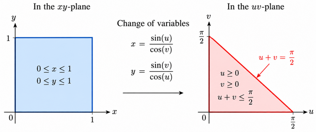
    Now comes the surprising part. Introduce new variables u and v by

    x = sin(u) cos(v) , y = sin(v) cos(u) .

    The square

    0≤x≤1 , 0≤y≤1

    corresponds to the triangular region

    u≥0 , v≥0 , u+v ≤ π2 .

    To see where the last boundary comes from, notice that

    x≤1 ⇔ sin(u) ≤ cos(v) ⇔ u+v ≤ π2 ,

    and the condition on y gives the same inequality.

    The Jacobian

    We compute

    ∂x∂u = cos(u) cos(v) , ∂x∂v = sin(u) sin(v) cos(v) 2 .

    Similarly,

    ∂y∂u = sin(u) sin(v) cos(u) 2 , ∂y∂v = cos(v) cos(u) .

    After simplifying the determinant, the Jacobian is

    ∂(x,y) ∂(u,v) = 1 − x2 y2 .

    This is exactly the expression that appears in the denominator of our original integral. Therefore,

    dxdy 1 − x2 y2 = dudv .

    The complicated-looking integrand has completely disappeared.

    The integral becomes an area

    Our double integral is now simply

    I = ∫ 0 π2 ∫ 0 π2 − u dv du .

    Geometrically, this is the area of a right triangle whose two perpendicular sides both have length

    π2

    Therefore,

    I = 12 · π2 · π2 = π2 8 .

    We have proved that

    1 + 132 + 152 + 172 + ⋯ = π2 8 .

    Recovering the full series

    Let

    T = ∑ n=1 ∞ 1 n2 .

    Split the series into its odd and even terms. The odd terms have sum

    π2 8

    while the even terms have sum

    122 + 142 + 162 + ⋯ = 14 T .

    Consequently,

    T = π2 8 + 14 T .

    Thus,

    34 T = π2 8 ,

    and finally,

    T = π2 6 .

    Why this proof is remarkable

    We started with an infinite series involving nothing but reciprocals of squares. We then represented part of that series by a double integral over a square. A carefully chosen trigonometric change of variables transformed the square into a triangle and, at the same time, made the integrand disappear.

    The infinite series was therefore reduced to the area of a triangle:

    12 · π2 · π2 = π2 8 .

    From there, separating the odd and even terms gives the celebrated result

    ∑ n=1 1 n2 = π2 6 .

    It is a striking example of how an infinite series, a double integral, a trigonometric substitution, and a simple geometric area can all describe the same number.


    Another Problem Where Two Dimensions Help

    The double-integral proof of the Basel sum illustrates a powerful mathematical idea: sometimes a problem becomes easier when we move to a higher dimension.

    One of the most beautiful examples is the Gaussian integral. A one-dimensional integral that resists ordinary antiderivative methods becomes accessible after it is squared and transformed into a two-dimensional integral.

    Continue exploring: The Gaussian Integral and Beyond: From e^(-x²) to a Family of Integrals

    Long before Euler solved the Basel problem, ancient Greek mathematicians had developed ingenious geometric methods for evaluating infinite sums. In particular, Archimedes used areas of triangles to establish a remarkable infinite series identity. Discover his method in How the Ancient Greeks Summed Infinite Series Without Calculus .

  • Why the Equilateral Triangle Wins: Maximum Area for a Fixed Perimeter

    Suppose you have a fixed length of wire and want to bend it into a triangle. Which triangle encloses the largest possible area?

    It is natural to guess that the answer is the equilateral triangle. But why? This is a beautiful example of how a geometric optimization problem can be turned into a multivariable calculus problem and solved using Lagrange multipliers.

    Setting up the problem

    Let the side lengths of the triangle be

    a, b, c.

    Suppose the perimeter is fixed and equal to P. Thus,

    a+b+c = P.

    We want to determine which values of a, b, and c produce the largest possible area.

    Heron’s formula

    Let

    s = P 2

    be the semiperimeter. Heron’s formula can be written in squared form as

    A 2 = s ( s−a ) ( s−b ) ( s−c ) .

    Because the perimeter is fixed, s is also fixed. Moreover, maximizing A is equivalent to maximizing A2. So this form of Heron’s formula is particularly convenient for our problem.

    A useful change of variables

    Introduce three new variables:

    x=s−a, y=s−b, z=s−c.

    The triangle inequalities imply that x, y, and z are positive.

    Adding the three equations gives

    x+y+z = 3s − ( a+b+c ) .

    Since

    a+b+c = 2s,

    we obtain the simple constraint

    x+y+z = s.

    Heron’s formula now becomes

    A 2 = sxyz.

    Since s is fixed, maximizing the area is equivalent to maximizing

    f ( x,y,z ) = xyz

    subject to

    x+y+z = s.

    The original geometry problem has therefore become a simple question: among three positive numbers with a fixed sum, when is their product largest?

    Using Lagrange multipliers

    Define

    f ( x,y,z ) = xyz

    and let the constraint function be

    g ( x,y,z ) = x+y+z.

    At a constrained maximum, the gradients of f and g must be parallel:

    ∇f = λ ∇g.

    We have

    ∇f = ⟨ yz, xz, xy ⟩

    and

    ∇g = ⟨ 1, 1, 1 ⟩.

    Therefore, the Lagrange multiplier equations are

    yz=λ, xz=λ, xy=λ.

    Thus,

    yz = xz = xy.

    Since x, y, and z are positive, these equations imply

    x = y = z.

    Their sum is s, so

    x = y = z = s 3 .

    Returning to the triangle

    Recall that

    x=s−a, y=s−b, z=s−c.

    Since x=y=z , we obtain

    a = b = c.

    Because the perimeter is P, each side must therefore have length

    a = b = c = P 3 .

    Therefore, the triangle of maximum area is the equilateral triangle.

    What is the maximum area?

    For an equilateral triangle with side length P 3 , the area is

    A max = 3 4 ( P 3 ) 2 .

    Therefore,

    A max = 3 P 2 36 .

    Why this argument is interesting

    We started with a geometric question about triangles. Heron’s formula converted the area problem into an algebraic one. A simple change of variables then transformed it into the problem of maximizing the product of three positive numbers whose sum is fixed.

    Lagrange multipliers reveal the symmetry automatically: at the maximum, the three variables must be equal. Translating that condition back into geometry tells us that the three sides of the triangle must also be equal.

    This is one of the appealing features of multivariable calculus: a geometric statement that seems intuitively obvious emerges naturally from an optimization calculation.

    Conclusion: Among all triangles with a fixed perimeter, the equilateral triangle has the largest area.

    For another surprising connection between equilateral-triangle geometry and a classical geometric object, see The Steiner Inellipse and a Surprising Area Characterization .

    The equilateral triangle is distinguished by its symmetry. In three dimensions, the regular tetrahedron has similar geometric elegance. Explore its face areas, volume, and a three-dimensional Pythagorean theorem in The Geometry of a Tetrahedron .

  • The Gaussian Integral and Beyond: From e^(-x²) to a Family of Integrals

    Some integrals are easy to write down but surprisingly difficult to evaluate. One of the most famous examples is

    ∫−∞∞ e−x2 dx .

    The function e−x2 has no elementary antiderivative. Yet the improper integral has the remarkably simple value

    ∫−∞∞ e−x2 dx = π .

    Even more interesting is the method used to obtain this result. By turning a one-dimensional integral into a two-dimensional one, we can exploit geometry. Once we understand that idea, it leads naturally to integrals involving e−x4, e−xp, and even integrals in which the Gaussian is multiplied by a sine or cosine.

    Example 1: The Gaussian integral

    Let

    I = ∫0∞ e−x2 dx .

    Instead of trying to find an antiderivative, square the integral:

    I2 = ( ∫0∞ e−x2 dx ) ( ∫0∞ e−y2 dy ) .

    Thus,

    I2 = ∫0∞ ∫0∞ e − ( x2 + y2 ) dxdy .

    Now something important has happened. The expression

    x2 + y2

    suggests polar coordinates. In the first quadrant,

    x=rcos⁡ (θ) , y=rsin⁡ (θ) .

    Here

    0≤r<∞ , 0≤θ≤ π2 .

    Since

    dxdy = rdrdθ ,

    we obtain

    I2 = ∫0π2 ∫0∞ e−r2 rdrdθ .

    The radial integral is elementary:

    ∫0∞ e−r2 rdr = 12 .

    Therefore,

    I2 = π2 · 12 = π4 ,

    and hence

    ∫0∞ e−x2 dx = π2 .

    By symmetry,

    ∫−∞∞ e−x2 dx = π .

    The essential idea was not integration by parts or an ingenious substitution. It was to increase the dimension.

    Example 2: Changing the scale

    Consider

    ∫0∞ e−ax2 dx , a>0 .

    Let

    u=ax .

    Then

    dx = dua ,

    so

    ∫0∞ e−ax2 dx = 1a ∫0∞ e−u2 du = π2a .

    One geometric calculation has already produced an entire family of integrals.

    Example 3: An integral involving e−x4

    First consider

    ∫0∞ x3 e−x4 dx .

    The substitution u=x4 works immediately because

    du = 4x3dx .

    Hence,

    ∫0∞ x3 e−x4 dx = 14 ∫0∞ e−u du = 14 .

    Now remove the factor x3.

    Example 4: What about e−x4 itself?

    Consider

    J= ∫0∞ e−x4 dx .

    Let u=x4. Then

    dx = 14 u−34 du ,

    and therefore

    J = 14 ∫0∞ u−34 e−u du .

    This integral is not elementary, but it is a standard special function. The Gamma function is defined, for s>0, by

    Γ (s) = ∫0∞ us−1 e−u du .

    Therefore,

    ∫0∞ e−x4 dx = 14 Γ ( 14 ) .

    The Gaussian was already hiding the Gamma function

    Apply the same substitution to the Gaussian integral. With u=x2,

    ∫0∞ e−x2 dx = 12 Γ ( 12 ) .

    But our two-dimensional calculation showed that the same integral equals π2. Consequently,

    Γ ( 12 ) = π .

    From e−x2 to e−xp

    Now consider the general integral

    Ip = ∫0∞ e−xp dx , p>0 .

    Set u=xp. Then

    dx = 1p u 1p −1 du .

    Therefore,

    Ip = 1p ∫0∞ u 1p −1 e−u du .

    By the definition of the Gamma function,

    ∫0∞ e−xp dx = 1p Γ ( 1p ) .

    Using the identity Γ ( s+1 ) = s Γ (s) , we can also write

    ∫0∞ e−xp dx = Γ ( 1+1p ) .

    For example,

    ∫0∞ e−x dx =1, ∫0∞ e−x2 dx = π2 , ∫0∞ e−x3 dx = 13 Γ ( 13 ) , ∫0∞ e−x4 dx = 14 Γ ( 14 ) .

    An even larger family

    We can include a power of x. Consider

    ∫0∞ xq e−xp dx ,

    where p>0 and q>−1. Again let u=xp. The same substitution gives

    ∫0∞ xq e−xp dx = 1p Γ ( q+1 p ) .

    For example,

    ∫0∞ x e−x4 dx = 14 Γ ( 12 ) = π4 ,

    while

    ∫0∞ x3 e−x4 dx = 14 Γ (1) = 14 .

    Thus three very similar-looking integrals can have rather different-looking answers:

    ∫0∞ e−x4 dx = 14 Γ ( 14 ) , ∫0∞ x e−x4 dx = π4 , ∫0∞ x3 e−x4 dx = 14 .

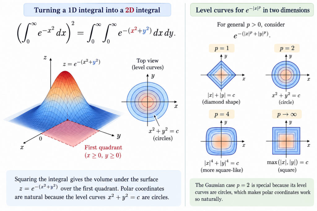
    Why did circles appear?

    There is a geometric reason the Gaussian calculation worked so beautifully. When we squared the Gaussian integral, the exponent became

    x2 + y2 .

    The level curves

    x2 + y2 = c

    are circles. Polar coordinates are therefore perfectly adapted to the problem.

    If instead we square ∫0∞ e−x4 dx , we obtain

    ∫0∞ ∫0∞ e − ( x4 + y4 ) dxdy .

    The corresponding level curves are

    x4 + y4 = c .

    They are not circles. More generally, e−xp is naturally connected with regions of the form

    |x|p + |y|p ≤ rp .

    For p=2, these are ordinary disks. For larger values of p, their boundaries become increasingly square-like. The Gaussian is the particularly beautiful case in which the geometry becomes ordinary Euclidean geometry.

    A surprising turn: add a cosine

    Consider

    C (b) = ∫0∞ e−x2 cos⁡ (bx) dx .

    The answer is

    C (b) = π2 e − b24 .

    This is remarkable: multiplying a Gaussian by an oscillating cosine produces another Gaussian, now as a function of the parameter b.

    Here is a calculus derivation. Differentiate with respect to b:

    C′ (b) = − ∫0∞ x e−x2 sin⁡ (bx) dx .

    Since

    x e−x2 = − 12 ddx ( e−x2 ) ,

    integration by parts gives

    C′ (b) = − b2 C (b) .

    Therefore,

    C′ (b) C (b) = − b2 .

    Integrating gives

    C (b) = A e − b24 .

    At b=0,

    C (0) = ∫0∞ e−x2 dx = π2 .

    Thus,

    ∫0∞ e−x2 cos⁡ (bx) dx = π2 e − b24 .

    For example, taking b=2 gives

    ∫0∞ e−x2 cos⁡ (2x) dx = π2e .

    What happens with sine?

    Now consider

    S (b) = ∫0∞ e−x2 sin⁡ (bx) dx .

    Unlike the cosine integral, this does not reduce to an elementary expression involving only exponentials and π. It can be written using a special function called Dawson’s integral,

    F (z) = e−z2 ∫0z et2 dt .

    The result is

    ∫0∞ e−x2 sin⁡ (bx) dx = F ( b2 ) .

    The difference between sine and cosine has a simple symmetry explanation. The function

    e−x2 cos⁡ (bx)

    is even, while

    e−x2 sin⁡ (bx)

    is odd. Therefore, over the entire real line,

    ∫−∞∞ e−x2 sin⁡ (bx) dx = 0 ,

    whereas

    ∫−∞∞ e−x2 cos⁡ (bx) dx = π e − b24 .

    One function keeps returning

    We started with e−x2. It has no elementary antiderivative, so at first it seems difficult to work with. But instead of disappearing, the Gaussian keeps returning.

    Geometry gives

    ∫−∞∞ e−x2 dx = π .

    The Gamma function places it inside the larger family

    ∫0∞ e−xp dx = Γ ( 1+1p ) .

    Adding a power of x produces

    ∫0∞ xq e−xp dx = 1p Γ ( q+1 p ) .

    And adding an oscillating cosine gives another Gaussian:

    ∫−∞∞ e−x2 cos⁡ (bx) dx = π e − b24 .

    This last identity is a glimpse of a much deeper fact: under the Fourier transform, the Gaussian essentially transforms into itself.

    So a single integral that cannot be evaluated by ordinary antiderivatives opens the door to geometry, the Gamma function, differential equations, generalized Lp geometry, and Fourier analysis.

    Sometimes an integral becomes easier not by finding a better antiderivative, but by finding a larger mathematical structure around it.

    From one dimension to two: squaring the Gaussian integral reveals circular level curves, making polar coordinates the natural choice.

    Another Famous Improper Integral

    The Gaussian integral shows how an integral over an infinite interval can be evaluated by introducing an extra dimension and exploiting symmetry. Another celebrated improper integral has a very different appearance:

    ∫ 0 ∞ sin ⁡ ( a x ) x d x = π 2 , a > 0 .

    What is especially surprising is that the answer does not depend on the positive parameter a .

    Continue exploring: A Surprising Improper Integral: Why the Integral of sin(ax)/x Is Always π/2


    Another Problem Where Two Dimensions Help

    The Gaussian integral becomes manageable after a surprising change of viewpoint: instead of attacking a one-dimensional integral directly, we square it, create a double integral, and use two-dimensional geometry.

    The same general idea appears in a completely different problem. The famous series 1 + 14 + 19 + ⋯ can also be approached through a double integral.

    Continue exploring: Proving 1 + 1/4 + 1/9 + ⋯ = π²/6 with a Double Integral


    From the Gaussian Integral to a Real Signal

    The Gaussian function is much more than an elegant calculus example. Gaussian distributions arise naturally when many small independent effects are added together, which makes them fundamental in probability, statistics, physics, and engineering.

    A particularly interesting example appears in OFDM communication signals. The in-phase and quadrature components become approximately Gaussian, but the signal magnitude follows a different distribution: the Rayleigh distribution.

    Continue exploring: Why Does an OFDM Signal Have a Rayleigh Distribution?

  • When Does x cos(x) Take the Same Value Twice?

    Consider the function

    f(x) = xcos(x)

    on the interval

    0≤x≤ π2.

    At both ends of the interval the function is zero:

    f(0) = f ( π2 ) =0.

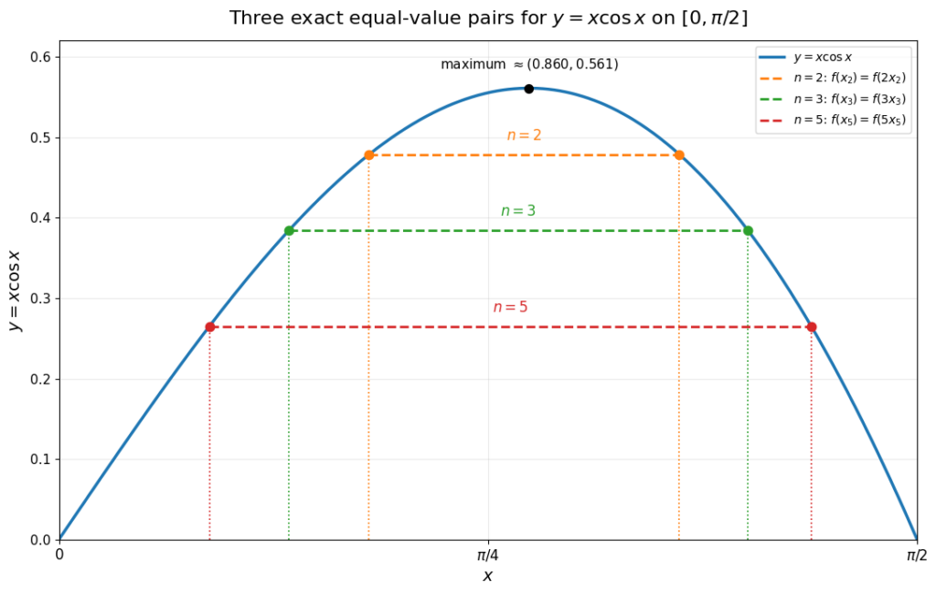
    Between these endpoints, the function rises to a single maximum and then falls back to zero. This means that every value strictly between zero and the maximum is attained at exactly two points.

    Why is there only one maximum?

    Differentiate:

    f′ (x) = cos(x) − xsin(x).

    At an interior critical point,

    cos(x) = xsin(x),

    or equivalently,

    xtan(x) =1.

    The function x tan(x) is strictly increasing on ( 0, π2 ) because

    ddx [ xtan(x) ] = tan(x) + x sec2 (x) >0.

    Therefore the equation xtan(x) =1 has exactly one solution. Numerically,

    x≈0.8603335890,

    and the maximum value is approximately

    fmax ≈0.5610963382.

    The main idea

    Usually, finding the two points at which xcos(x) has the same value leads to a transcendental equation. But something interesting happens if the second point is an integer multiple of the first.

    Suppose the two points are x and nx, where n>1 is an integer. To keep both points inside the interval, we require

    0<x< π2n.

    We want

    f(x) = f(nx).

    Thus

    xcos(x) = nx cos(nx).

    Since x>0, we can divide by x:

    cos(x) = ncos(nx).

    This is where Chebyshev polynomials enter the problem.

    What is a Chebyshev polynomial?

    The Chebyshev polynomial of the first kind, denoted by Tn, is defined by the identity

    Tn ( cosθ ) = cos(nθ).

    For example,

    T2 (c) = 2c2 −1, T3 (c) = 4c3 −3c,

    and

    T5 (c) = 16c5 − 20c3 + 5c.

    Now set

    c= cos(x).

    Then

    cos(nx) = Tn (c),

    so our transcendental equation becomes the algebraic equation

    c= n Tn (c).

    This is the key observation: a question about two equal values of a transcendental function has turned into a polynomial equation.

    Case 1: n = 2

    We have

    c= 2 ( 2c2 −1 ).

    Therefore

    4c2 −c−2 =0.

    The root satisfying the required interval condition is

    c= 1+33 8 .

    Hence

    x= arccos ( 1+33 8 ).

    The two different inputs x and 2x therefore give exactly the same value of xcos(x) .

    Case 2: n = 3

    Now

    c= 3 ( 4c3 −3c ).

    Since c is positive, division by c gives

    1= 12c2 −9.

    Thus

    c2 = 56,

    and therefore

    x= arccos ( 56 ).

    So x and 3x give another exact pair with the same value of the function.

    Case 3: n = 5

    Using

    T5 (c) = 16c5 − 20c3 + 5c,

    the equation c= 5 T5 (c) becomes, after dividing by c,

    20c4 − 25c2 +6 =0.

    Setting u=c2 gives

    20u2 − 25u +6 =0.

    Therefore

    u = 25±145 40 .

    However, not both algebraic roots correspond to our original problem. We need

    0<x< π10,

    so c= cos(x) > cos ( π10 ). Only the larger root satisfies this condition. Hence

    c = 25+145 40 ,

    and

    x= arccos ( 25+145 40 ).

    Thus x and 5x form a third exact pair.

    What makes this interesting?

    The graph tells us immediately that xcos(x) takes most of its values twice. But the locations of those two points are usually not available in closed form.

    Requiring the two inputs to have the special form x and nx changes the problem completely. The multiple-angle identity

    cos(nx) = Tn ( cos(x) )

    turns the transcendental equation into a polynomial equation. For n=2,3,5 , that polynomial equation gives particularly clean exact answers.


    A Related Same-Value Problem

    The function x ⁢ cos ⁡ ( x ) leads to one kind of same-value problem. A surprisingly different example appears when we ask the same question about x 1 / x .

    Continue exploring: When Does x^(1/x) Take the Same Value Twice?

  • A Surprising Integral on the Sphere: Why Every Direction Is the Same

    Consider the integral

    I ( u ) = ∫ S n − 1 | u · x | d S ( x )

    where S n − 1 is the unit sphere in R n and u is a fixed vector. At first glance, this looks like a difficult high-dimensional integral. The absolute value creates a nonsmooth integrand, but the symmetry of the sphere makes the calculation surprisingly simple.

    The key observation

    Write

    u = ∥ u ∥ e

    where e is a unit vector. Then

    | u · x | = ∥ u ∥ | e · x |

    Therefore,

    I ( u ) = ∥ u ∥ ∫ S n − 1 | e · x | d S ( x )

    The remaining integral does not depend on the direction of e. The sphere is rotationally symmetric, so we may rotate the coordinate system and assume that

    e = ( 1 , 0 , … , 0 )

    Then

    e · x = x 1

    and therefore

    I ( u ) = ∥ u ∥ ∫ S n − 1 | x 1 | d S ( x )

    A geometric interpretation

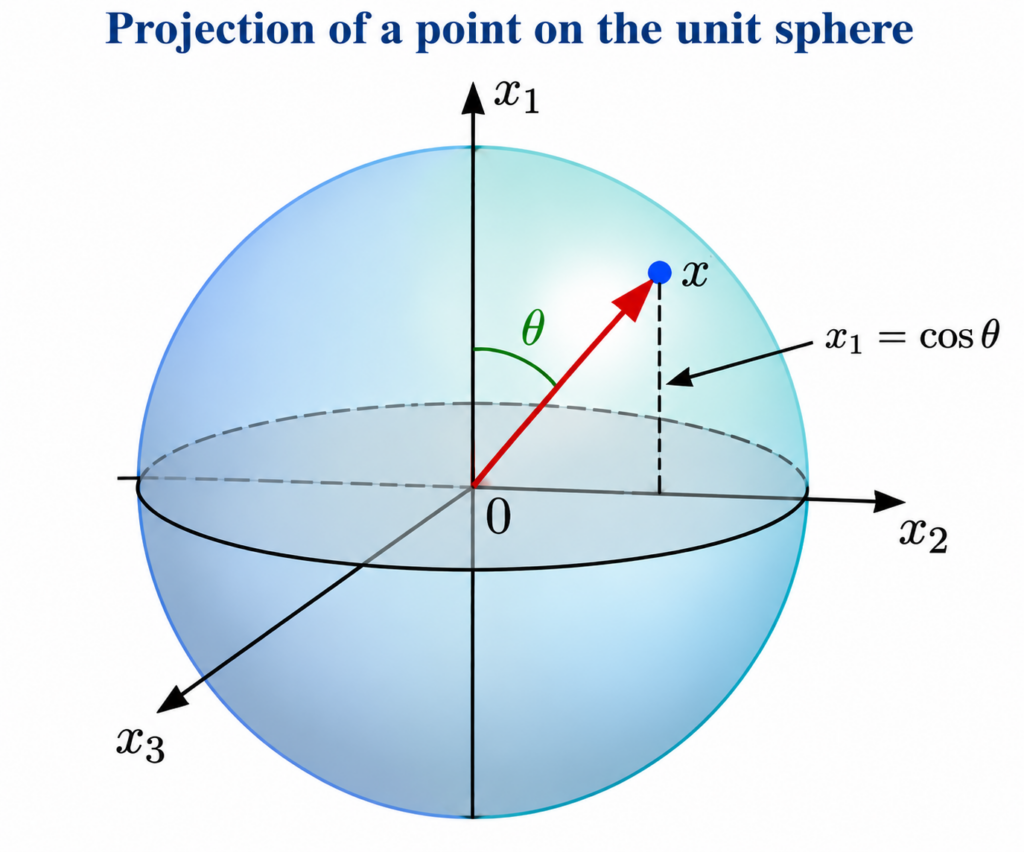
    For a point x on the sphere, let θ be the angle between x and the chosen direction e . Then the projection of x onto this direction is

    e · x = cos ( θ )

    so

    | u · x | = ∥ u ∥ | cos ( θ ) |

    The integral is therefore the total absolute projection of all points on the sphere onto a fixed direction.

    Measuring spheres

    The notation | S n | means the surface area of the unit sphere S n .

    For example,

    • S 0 consists of two points, so | S 0 | = 2 .
    • S 1 is the unit circle, so | S 1 | = 2 π .
    • S 2 is the ordinary unit sphere, so | S 2 | = 4 π .

    Now consider the sphere S n − 1 . Fix the angle θ between a point x on this sphere and a fixed direction e .

    All points with the same angle θ form a lower-dimensional sphere S n − 2 . Therefore, | S n − 2 | is the surface area of this slice of the sphere.

    This is the geometric reason that | S n − 2 | appears when we compute the integral using spherical coordinates.

    The lower-dimensional sphere

    To compute the integral, we slice the sphere by fixing the angle θ . Each slice is itself a sphere of one lower dimension.

    The notation

    | S n − 2 |

    means the surface area of the unit sphere S n − 2 one dimension lower. For example,

    • |S0|=2, because it consists of two points;
    • |S1|=2π, because it is the unit circle;
    • |S2|=4π, because it is the usual sphere.

    Using spherical coordinates, the surface element becomes

    dS = sin ( θ ) n − 2 dθ d S n − 2

    Therefore,

    ∫ S n − 1 | x 1 | dS = 2 | S n − 2 | ∫ 0 π/2 cos ( θ ) sin ( θ ) n − 2 dθ

    Finishing the computation

    The remaining one-dimensional integral is elementary. Let

    y = sin ( θ )

    so that

    dy = cos ( θ ) dθ

    Therefore,

    ∫ 0 π/2 cos ( θ ) sin ( θ ) n − 2 dθ = ∫ 0 1 y n − 2 dy = 1 n − 1

    Substituting this result gives

    ∫ S n − 1 | x 1 | dS = 2 | S n − 2 | n − 1

    Finally,

    ∫ S n − 1 | u · x | dS = 2 | S n − 2 | n − 1 ‖ u ‖

    Examples

    The formula becomes especially simple in low dimensions.

    The circle S 1

    For the unit circle we have n = 2 . The lower-dimensional sphere is

    S 0

    which consists of two points, so

    | S 0 | = 2

    Therefore,

    ∫ S 1 | u · x | d S = 2 · 2 1 ‖ u ‖ = 4 ‖ u ‖

    The sphere S 2

    For the ordinary unit sphere in R 3 we have

    n = 3

    and the lower-dimensional sphere is the unit circle:

    | S 1 | = 2 π

    Hence,

    ∫ S 2 | u · x | d S = 2 · 2 π 2 ‖ u ‖ = 2 π ‖ u ‖

    In both examples, the direction of u does not matter. Only its length remains. This is a direct consequence of the rotational symmetry of the sphere.

    The main idea

    The calculation is simple because the sphere has no preferred direction. A rotation can move any vector u to a coordinate axis without changing the geometry of the sphere.

    Therefore, the integral depends only on the length of the vector:

    ∫ S n − 1 | u · x | d S = C ( n ) ‖ u ‖

    where C ( n ) is a constant that depends only on the dimension.

    The important lesson is not the integration itself, but the symmetry behind it: whenever a problem on a sphere involves a single fixed vector, the first question should be whether a rotation can remove the direction completely.

  • Gabriel’s Horn: When Can an Infinite Horn Be Painted?

    Can a shape stretch forever, hold a finite amount of liquid, and still have an infinite surface to paint? Gabriel’s horn does exactly that. The more interesting question is what can happen for other horns. Can we classify every possibility?

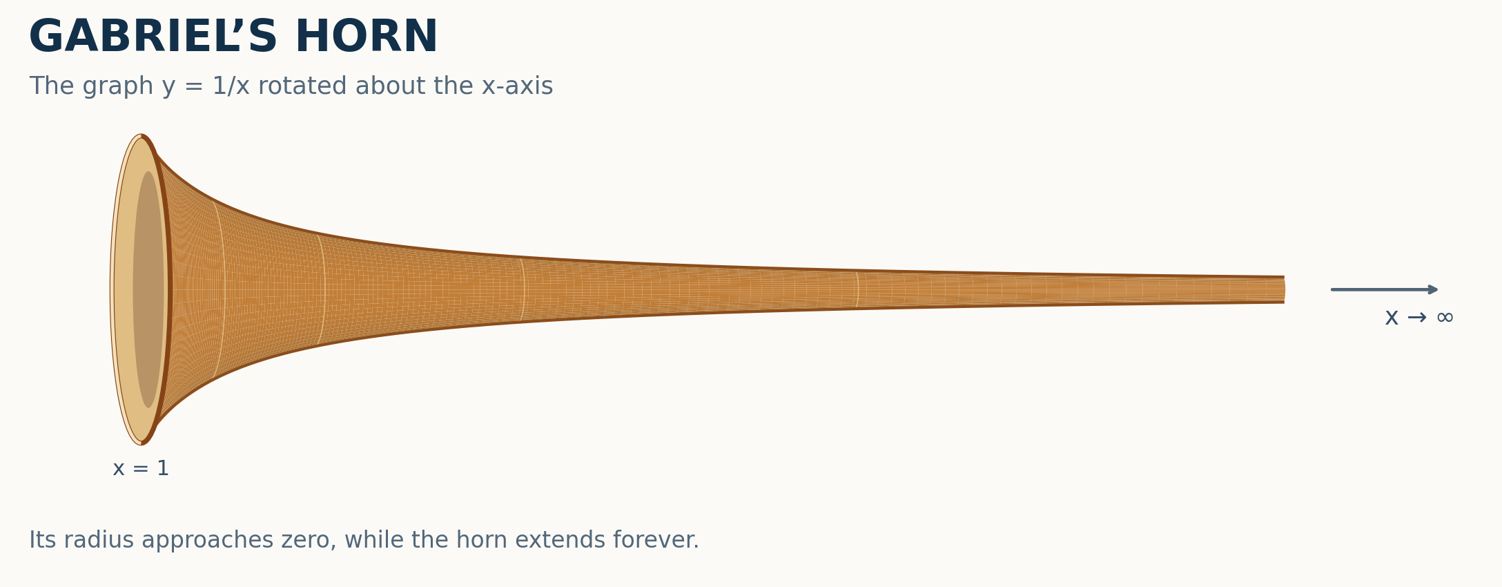
    Illustration of Gabriel’s horn, formed by rotating y equals one over x for x at least one about the x-axis. Its circular opening is wide at x equals one; the radius narrows as the horn continues indefinitely to the right.
    Gabriel’s horn is generated by rotating the graph of y = 1/x for x ≥ 1 about the x-axis. The illustration shows only a finite portion.

    The familiar paradox

    At position x, the horn has radius 1/x. The disk method gives its volume:

    V=π∫1∞1x2dx=πV=\pi\int_1^\infty\frac{dx}{x^2}=\pi

    But the lateral surface area satisfies

    S=2π∫1∞1x1+1x4dxS≥2π∫1∞1xdx=∞

    So the horn can be filled with π cubic units, although painting its entire outside would require infinite area. This is the usual painter’s paradox. [1, 2]

    A general horn

    Now let f be a nonnegative continuously differentiable function on [a, ∞), and rotate the region under its graph about the x-axis. “Painting” means covering the curved lateral surface; including the single disk at x = a changes no finite-versus-infinite result. The familiar formulas are [1]

    V=π∫a∞f⁡(x)2dxS=2π∫a∞f⁡(x)1+f′⁡(x)2dx

    To determine whether the second integral converges, use the elementary inequality

    max{1,|v|}≤1+v2≤1+|v|\max\{1,|v|\}\le\sqrt{1+v^2}\le1+|v|

    Apply it with v = f′(x), multiply by f(x) ≥ 0, and integrate. We obtain a useful if and only if statement:

    S<∞⇔∫a∞f⁡(x)dx<∞and∫a∞f⁡(x)|f′⁡(x)|dx<∞

    The first integral measures the radii accumulated along the axis. The second detects rapid changes in the radius. Both must be finite to paint the horn.

    The four possibilities

    VolumeLateral areaCondition
    FiniteFiniteBoth integrals in the painting test converge.
    FiniteInfiniteThe integral of f² converges, but at least one integral in the painting test diverges.
    InfiniteFiniteImpossible.
    InfiniteInfiniteThe integral of f² diverges.

    Why is the third row impossible? Since the derivative of f² is 2ff′, the painting test gives the bound

    f⁡(x)2≤f⁡(a)2+2∫a∞f⁡(x)|f′⁡(x)|dx

    Thus a paintable horn has a bounded radius. If M is an upper bound for f, then f² ≤ Mf. The painting test also says the integral of f is finite, so the integral of f² is finite. In short: every paintable horn is fillable. The converse fails, as Gabriel’s horn shows. The implication is also noted in a Calculus II laboratory abstract by Royer. [3]

    An entire family of examples

    Consider

    f(x)=1xp,x≥1,p>0f(x)=x^{-p},\qquad x\ge1,\quad p>0

    Here f(x) = x−p decreases from f(1) = 1 toward 0. Its derivative is negative, so |f′(x)| = −f′(x). Thus the second integral in the painting test is

    ∫1∞f⁡(x)|f′⁡(x)|dx=−∫1∞f⁡(x)f′⁡(x)dx

    Now (f(x)²)′ = 2f(x)f′(x). Integrating the expression on the right gives

    −∫1∞f⁡(x)f′⁡(x)dx=f(1)2−limx→∞f⁡(x)22=12.

    Therefore the second painting integral is finite for every p > 0. The volume is finite when 2p > 1, while the surface area is finite when p > 1.

    ExponentWhat happens?
    p > 1Both fillable and paintable.
    1/2 < p ≤ 1Fillable but not paintable; p = 1 is Gabriel’s horn.
    0 < p ≤ 1/2Neither fillable nor paintable.

    What if the horn wiggles?

    For a decreasing graph, the integral involving |f′| needs no separate test. For an oscillating graph, it really matters. Consider the smooth positive function

    f(x)=2+sin(x4)(1+x)2f(x)=\frac{2+\sin(x^4)}{(1+x)^2}

    The function is bounded above by 3/(1+x)², so both the integral of f and the volume integral of f² converge. Yet the oscillations become increasingly rapid. The term from differentiating sin(x⁴) makes f|f′| comparable, up to an integrable error, to |cos(x⁴)|/x. Substituting u = x⁴ shows that its integral diverges like the integral of |cos u|/u. Therefore this horn is fillable but not paintable even though the integral of its radii is finite.

    Gabriel’s horn fails the painting test because it shrinks too slowly. The oscillating horn fails because its surface becomes too corrugated. The two-integral criterion catches both.

    References

    1. Gilbert Strang and Edwin “Jed” Herman, Calculus Volume 1, OpenStax (2016), §6.2, “Determining Volumes by Slicing” and §6.4, “Arc Length of a Curve and Surface Area.”
    2. APEX Calculus, §7.4, “Arc Length and Surface Area,” Example 7.4.18 (Gabriel’s horn).
    3. Melvin G. Royer, “Gabriel’s Other Equipment,” abstract, Joint Mathematics Meetings (2010).

    Another Surprise from an Improper Integral

    Gabriel’s Horn shows how an improper integral can produce a result that seems geometrically impossible: a solid can have finite volume while its surface area is infinite.

    Improper integrals contain other surprises as well. One of the most famous is an oscillating integral involving sin ⁡ ( a x ) x , whose value turns out to be remarkably independent of a when a > 0 .

    Continue exploring: A Surprising Improper Integral: Why the Integral of sin(ax)/x Is Always π/2

  • When Does x^(1/x) Take the Same Value Twice?

    We begin with a simple equality:

    2 12 = 4 14 .

    The problem

    Consider the function f(x) = x 1x , x>0. The equality above shows that this function can take the same value at two distinct positive real numbers.

    x 1x = y 1y , x≠y, x>0, y>0.

    Prove that infinitely many such pairs exist, and describe all of them.

    Solution

    Consider the function f(x) = x 1x on [1,∞). It increases until x=e and then decreases toward 1. Thus, every horizontal line strictly between 1 and the maximum intersects the graph twice.

    Graph of f of x equals x to the power 1 over x The graph increases from the point 1 comma 1 to its maximum at x equals e, and then decreases toward 1. The horizontal line f of x equals 1.3 intersects the graph at approximately 1.471 and 7.857. x f(x) 1 f(x) = 1.3 maximum at x = e 1 e 1.471 7.857
    A horizontal line meets the graph twice. Here it gives the approximate pair (1.471,7.857).

    A parametrization of all pairs

    We now describe all the solutions. Assume first that x<y and set

    t = yx > 1.

    Then

    y=tx.

    Taking logarithms of x 1x = y 1y gives

    ln⁡x x = ln⁡(tx) tx .

    Multiplying by tx, we obtain

    tln⁡x = ln⁡x + ln⁡t.

    Therefore,

    (t−1) ln⁡x = ln⁡t,

    and hence

    x = t 1 t−1 .

    Since y = tx, it follows that

    y = t t t−1 .

    Thus, all solutions with x<y are given by

    (x,y) = ( t 1 t−1 , t t t−1 ) , t>1.

    Conversely, direct substitution shows that every t>1 produces a solution. Therefore, this parametrization gives every distinct pair with the smaller number written first. Reversing the two entries gives the solutions with x>y. Since there are infinitely many choices of t>1, there are infinitely many such pairs.

    A Few Examples

    Choosing t= n+1 n , n=1,2,3,…, gives the infinite family of rational solutions

    (x,y) = ( ( n+1 n ) n , ( n+1 n ) n+1 ).
    Examples from the rational family
    n t x y
    1 2 2 4
    2 3/2 9/4 27/8
    3 4/3 64/27 256/81
    4 5/4 625/256 3125/1024

    Approaching e

    These rational solutions approach e from opposite sides. Indeed, if

    xn = (1+ 1n) n , yn = (1+ 1n) n+1 ,

    then

    xn ↑ e and yn ↓ e.

    Thus, the smaller number in each pair approaches e from below, while the larger number approaches e from above.


    Another Same-Value Problem

    The function x 1 / x is not the only familiar-looking function that can take the same value at different inputs. A related question leads to a very different kind of equation.

    Continue exploring: When Does x cos(x) Take the Same Value Twice?