Author: anatoly

The Population Model That Fails—and Why Its Equation Is Everywhere: Population, Interest, and Radioactive Decay

“`html
A remarkably simple differential equation appears in many different places in the real world. We will begin with population growth. The first model we try will have a serious problem: it predicts unlimited growth. Fixing that problem will lead us to the logistic equation.

Then, surprisingly, we will return to our original equation and discover that it was not a bad equation at all. The same equation describes continuous compound interest, radioactive decay, and many other processes.

1. The Simplest Population Model

Let $P (t)$ denote a population at time $t$ .

One of the simplest assumptions we can make is this: the rate at which the population grows is proportional to the population itself.

$\frac{d P}{d t} = k P, P (0) = P_{0} .$

Here $k > 0$ is a constant. The idea seems reasonable. If there are twice as many individuals, we might expect approximately twice as many births. A larger population therefore grows faster.

The equation is separable:

$\frac{d P}{P} = k d t .$

Integrating gives

$\ln P = k t + C,$

and therefore

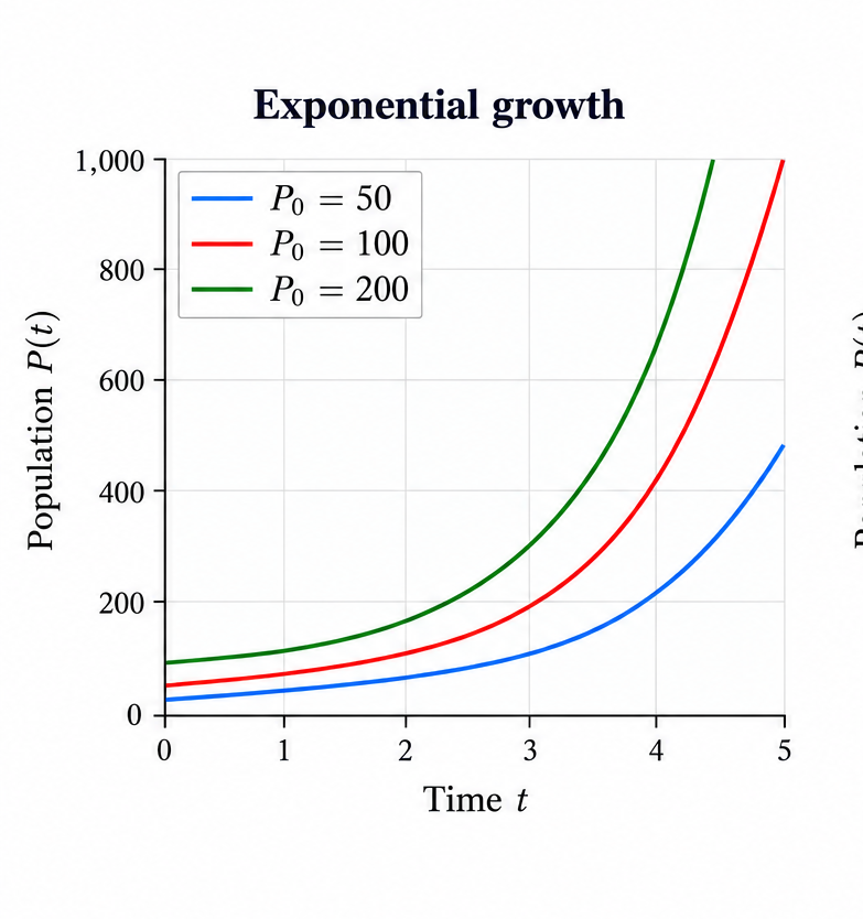
$P (t) = P_{0} e^{k t} .$

This is exponential growth.

There is an immediate problem. If $k > 0$ , then

$P (t) \to \infty as t \to \infty .$

According to this model, the population eventually becomes arbitrarily large. That cannot continue indefinitely in the real world. Food, water, space, and other resources are limited.

So our first population model is useful for describing growth over some periods, but it cannot be the whole story.
“`
“`html
2. Introducing a Carrying Capacity

Suppose the environment can sustainably support a maximum population $K$ . This number is called the carrying capacity.

We modify our original equation to

$\frac{d P}{d t} = k P (1 - \frac{P}{K})$

This is the logistic equation.

The new factor

$(1 - \frac{P}{K})$

is what changes everything. When the population is small compared with $K$ , this factor is close to 1, so the population behaves approximately like ordinary exponential growth. As the population becomes larger, the factor becomes smaller and the growth slows down.

We Can Predict the Solutions Without Solving the Equation

This is one of the most useful ideas in differential equations: we do not always need an explicit formula to understand what the solutions will do.

First suppose

$0 < P < K .$

Then

$(1 - \frac{P}{K}) > 0,$

and consequently

$\frac{d P}{d t} > 0 .$

So the population increases.

Now suppose $P = K$ . Then

$(1 - \frac{P}{K}) = 0,$

so

$\frac{d P}{d t} = 0 .$

The population remains constant at the carrying capacity.

Finally, if $P > K$ , then

$(1 - \frac{P}{K}) < 0,$

and therefore

$\frac{d P}{d t} < 0 .$

The population decreases toward the carrying capacity.

Where Is the Population Growing Fastest?

The growth rate is

$k P (1 - \frac{P}{K}) .$

As a function of $P$ , this is a downward-opening quadratic:

$k P - \frac{k P^{2}}{K} .$

Its maximum occurs at

$P = \frac{K}{2} .$

This tells us something important about the shape of the population curve.

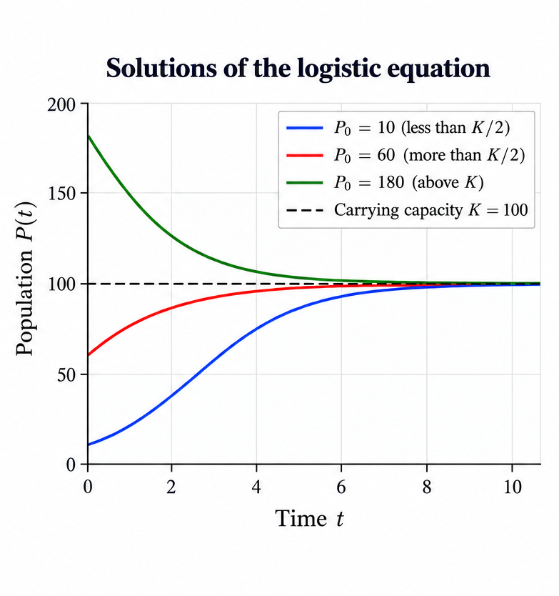
If $P_{0} < \frac{K}{2}$ , the population initially grows faster and faster. When it reaches $P = \frac{K}{2}$ , its growth rate is greatest. After that, the population continues to increase, but more and more slowly as it approaches $K$ . This produces the familiar S-shaped logistic curve.

If $\frac{K}{2} < P_{0} < K$ , the population begins above the point of fastest growth. It still increases toward $K$ , but it slows down from the beginning.

Finally, if $P_{0} > K$ , the population decreases toward $K$ .

Thus, before solving the logistic equation, we can already predict the three different types of solution curves shown in the next figure.
“`
“`html id=”p87fcf”
3. Now Let Us Solve the Logistic Equation

We now return to the logistic equation

$\frac{d P}{d t} = k P (1 - \frac{P}{K}), P (0) = P_{0} .$

We have already learned a great deal about its solutions without solving it. Now let us find the actual formula.

First separate the variables:

$\frac{d P}{P (1 - \frac{P}{K})} = k d t .$

Since

$\frac{1}{P (1 - \frac{P}{K})} = \frac{1}{P} + \frac{1}{K - P},$

we can integrate:

$\int (\frac{1}{P} + \frac{1}{K - P}) d P = \int k d t .$

This gives

$\ln P - \ln (K - P) = k t + C .$

Combining the logarithms,

$\ln (\frac{P}{K - P}) = k t + C .$

Exponentiating both sides gives

$\frac{P}{K - P} = C e^{k t} .$

Using the initial condition $P (0) = P_{0}$ , we obtain

$C = \frac{P_{0}}{K - P_{0}} .$

After solving for $P$ , we obtain the logistic growth formula:

$P (t) = \frac{K}{1 + \frac{K - P_{0}}{P_{0}} e^{- k t}} .$

Now the formula confirms what we predicted from the differential equation. For positive initial populations, the population approaches the carrying capacity:

$P (t) \to K as t \to \infty .$

So the carrying capacity is not merely a number inserted into the model. It becomes the long-term population predicted by the model.

4. Was Our Original Equation Really So Bad?

We rejected the equation

$\frac{d y}{d t} = k y$

as a model of population growth over an unlimited period of time. But the equation itself is one of the most important differential equations in mathematics.

The initial-value problem

$\frac{d y}{d t} = k y, y (0) = y_{0}$

has the solution

$y (t) = y_{0} e^{k t} .$

What changes from one application to another is the meaning of $y$ and the sign and meaning of the proportionality constant.

5. Continuous Compound Interest

Suppose an amount of money $A (t)$ earns interest continuously at an annual rate $r$ . The rate at which the account balance changes is proportional to the amount currently in the account:

$\frac{d A}{d t} = r A, A (0) = A_{0} .$

Therefore,

$A (t) = A_{0} e^{r t} .$

The same equation that produced exponential population growth now describes the growth of money.

6. Radioactive Decay

Now consider a radioactive substance. The more radioactive nuclei that are present, the more nuclei are available to decay. Thus, the magnitude of the decay rate is proportional to the amount currently present.

This time the quantity is decreasing, so we write

$\frac{d N}{d t} = - λ N, N (0) = N_{0},$

where $λ > 0$ is the decay constant.

The solution is

$N (t) = N_{0} e^{- λ t} .$

7. One Equation, Many Processes

We began with perhaps the simplest population model imaginable: the rate of change of a population is proportional to the population itself.

As a long-term population model, it failed. Unlimited exponential population growth is impossible in an environment with limited resources.

Introducing a carrying capacity led naturally to the logistic equation. Even more importantly, we were able to predict the behavior of its solutions before solving the equation.

But our original equation was far from useless. The same basic mathematical law appears in continuous compound interest and radioactive decay.

The common idea is simple:

The rate of change of a quantity is proportional to the amount of that quantity currently present.

Population, money, and radioactive atoms seem like completely different things. Mathematically, however, they can obey the same law.

That is one of the remarkable features of differential equations: the same mathematical equation can describe very different processes in the real world.

Related: See another example where a simple mathematical model produces a surprising—and ultimately unrealistic—prediction: A Sliding Ladder: Is It Better to Slide or Jump? .

October 2, 2026
How Do You Fit a Cylinder to Thousands of Points in Real Time?

Several years ago, I was given a practical geometry problem:

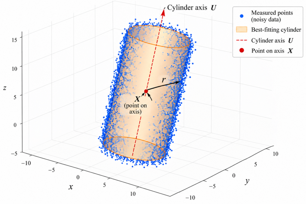
Given thousands of measured points in three-dimensional space, find the cylinder that best fits them.

There was an additional requirement that made the problem much more interesting. The calculation had to be fast enough to operate in real time.

This meant that simply defining a mathematically reasonable fitting problem was not enough. The equations had to be arranged so that thousands of data points could be processed efficiently, the derivatives could be evaluated quickly, and each optimization step would require solving only a very small system of equations.

The resulting method combines geometry, calculus, least squares, and the Gauss–Newton method.

The Geometry of a Cylinder

Suppose that

$X = {(x_{1}, x_{2}, x_{3})}^{T}$

is a point on the axis of a cylinder, and

$U = {(u_{1}, u_{2}, u_{3})}^{T}$

is a vector pointing along the axis.

Let $P$ be a point on the surface of the cylinder.

The defining geometric property is simple:

The perpendicular distance from every point on the cylinder to its axis is the radius $r$ .

Distance from a Point to the Axis

Consider the vector

$P - X .$

Part of this vector points along the cylinder axis, while the remaining part is perpendicular to the axis.

If $α$ is the angle between $P - X$ and $U$ , then

$‖ P - X ‖ sin α = r .$

Squaring gives

${‖ P - X ‖}^{2} {sin α}^{2} = r^{2} .$

The dot product gives

${({(P - X)}^{T} U)}^{2} = {‖ P - X ‖}^{2} {‖ U ‖}^{2} {cos α}^{2} .$

Combining these relations eliminates the angle completely and gives

${‖ P - X ‖}^{2} - \frac{{({(P - X)}^{T} U)}^{2}}{{‖ U ‖}^{2}} = r^{2} .$

This is the equation we need.

The first term measures the squared distance from $X$ to $P$ . The fraction subtracts the squared component parallel to the axis. What remains is exactly the squared perpendicular distance to the axis.

Turning the Geometry into a Residual

Measured points will not lie exactly on a perfect cylinder.

For a measured point $P$ , define

$R (P) = {‖ P - X ‖}^{2} - \frac{{({(P - X)}^{T} U)}^{2}}{{‖ U ‖}^{2}} - r^{2} .$

For a point exactly on the cylinder,

$R (P) = 0 .$

For a noisy measured point, the residual will usually be nonzero.

Reducing the Number of Unknowns

At first the cylinder appears to have seven parameters: three coordinates for a point on its axis, three coordinates for the axis direction, and the radius.

But there is redundancy.

Moving the reference point $X$ along the axis does not change the cylinder. Also, multiplying $U$ by a nonzero constant does not change its direction.

Assuming the cylinder axis is not parallel to the $(x_{1}, x_{2})$ plane, choose

$X = {(x_{1}, x_{2}, 0)}^{T}, U = {(u_{1}, u_{2}, 1)}^{T} .$

Now the entire cylinder is described by only five unknown numbers:

$S = {(x_{1}, x_{2}, u_{1}, u_{2}, r)}^{T} .$

Two numbers locate the axis, two determine its direction, and one gives the radius.

From Geometry to Least Squares

Suppose our measuring system produces $m$ points:

$P_{1}, P_{2}, \dots, P_{m} .$

Each point produces a residual $R_{j}$ .

We find the best-fitting cylinder by minimizing

$f (S) = \frac{1}{2} \sum_{j = 1}^{m} R_{j}^{2} .$

This is a nonlinear least-squares problem.

Why the Derivatives Matter

Because the calculation had to run quickly, I derived the residual derivatives analytically.

For each measured point, we need derivatives with respect to the five unknown parameters:

$\nabla R = (\frac{\partial R}{\partial x_{1}}, \frac{\partial R}{\partial x_{2}}, \frac{\partial R}{\partial u_{1}}, \frac{\partial R}{\partial u_{2}}, \frac{\partial R}{\partial r}) .$

The formulas contain several repeated expressions. In an implementation, there is no reason to calculate the same quantity over and over.

For example, define

$q = \frac{(p_{1} - x_{1}) u_{1} + (p_{2} - x_{2}) u_{2} + p_{3}}{u_{1}^{2} + u_{2}^{2} + 1} .$

Then several derivative formulas become much shorter and faster to evaluate.

This may look like a minor algebraic simplification on paper. In a real-time numerical algorithm that evaluates the same expressions thousands of times, such simplifications matter.

The Jacobian

Collect all the residuals into the vector

$E = {(R_{1}, R_{2}, \dots, R_{m})}^{T} .$

The Jacobian $J$ has one row for every measured point and one column for every unknown parameter.

Therefore,

$J is an m \times 5 matrix.$

Gauss–Newton

The least-squares objective can be written compactly as

$f = \frac{1}{2} {‖ E ‖}^{2} .$

Its gradient is

$\nabla f = J^{T} E .$

Gauss–Newton approximates the Hessian by

$\nabla^{2} f \approx J^{T} J .$

At each iteration, instead of solving the original nonlinear problem from scratch, we solve

$J^{T} J G = - J^{T} E .$

The vector $G$ tells us how to change the current estimate of the cylinder.

Why Thousands of Points Are Not as Bad as They Sound

This is the computational feature that makes the method especially attractive.

Suppose the measuring system gives us 10,000 points.

Then $J$ has 10,000 rows.

But it still has only five columns.

Therefore,

$J^{T} J$

is only a

$5 \times 5$

matrix.

And

$J^{T} E$

contains only five numbers.

So although every iteration uses information from thousands of measured points, the linear system that determines the next step has only five unknowns.

That is a very useful structure for a real-time calculation.

Do Not Always Take the Full Step

A Gauss–Newton direction tells us which way to move, but taking the entire step is not always wise.

Write the update as

$S_{k + 1} = S_{k} + a_{k} G_{k}, 0 < a_{k} \leq 1 .$

The step length is chosen adaptively. Start with $a_{k} = 1$ and reduce it if necessary until the new point produces a sufficient decrease in the objective function.

In practice, the full step can often be accepted, but the line search gives the algorithm additional protection when the current estimate is not yet close to the solution.

When Do We Stop?

At a minimum we expect

$\nabla f = 0 .$

Numerically, we stop when

$‖ \nabla f ‖ < ε,$

where $ε$ is a small tolerance.

There is no benefit in demanding far more numerical precision than the data and the computer arithmetic can support. An unnecessarily small tolerance can even create numerical difficulties.

Did It Work?

Yes.

This was not a numerical example invented after the fact. The cylinder fitting problem came from a real application, and the algorithm had to work fast enough for real-time use.

The implementation worked extremely well.

What I found especially satisfying was that the final algorithm was built from familiar mathematical ingredients:

geometry → least squares → calculus → Gauss–Newton → real-time computation.

The important part was arranging those ingredients in the right way.

From Cylinders to Cones

A cylinder has constant radius. Once this fitting method works, a natural question is:

What happens if the radius changes as we move along the axis?

That leads to a cone.

The cone-fitting problem requires one additional parameter—the opening angle—and the derivatives become more complicated. But the central strategy remains the same:

choose an efficient geometric residual → derive its Jacobian → form a nonlinear least-squares problem → solve it with Gauss–Newton.

That will be the subject of the next post.

The Larger Lesson

There is an important distinction between solving a mathematical problem and solving it in a form that is useful in practice.

With 10,000 measured points, the original problem sounds large. But the geometry allows the unknown cylinder to be represented by only five parameters. Gauss–Newton then converts each iteration into a small five-variable linear problem.

This is one of the recurring ideas in applied mathematics:

A good mathematical formulation can be as important as the algorithm itself.

When the formulation is right, a problem involving thousands of three-dimensional measurements can become small enough to solve in real time.

A Closely Related Fitting Problem

Cylinder fitting is only one version of the real-time surface-fitting problem. A closely related challenge arises when the measured surface is a cone rather than a cylinder.

The change in geometry leads to a different mathematical problem, but the objective is the same: use the structure of the surface to obtain an accurate fit quickly enough for practical real-time computation.

Continue exploring: How Do You Fit a Cone to Thousands of Points in Real Time?

October 1, 2026
How Do You Fit a Cone to Thousands of Points in Real Time?

Several years ago, I was given an applied mathematics problem that sounded simple at first:

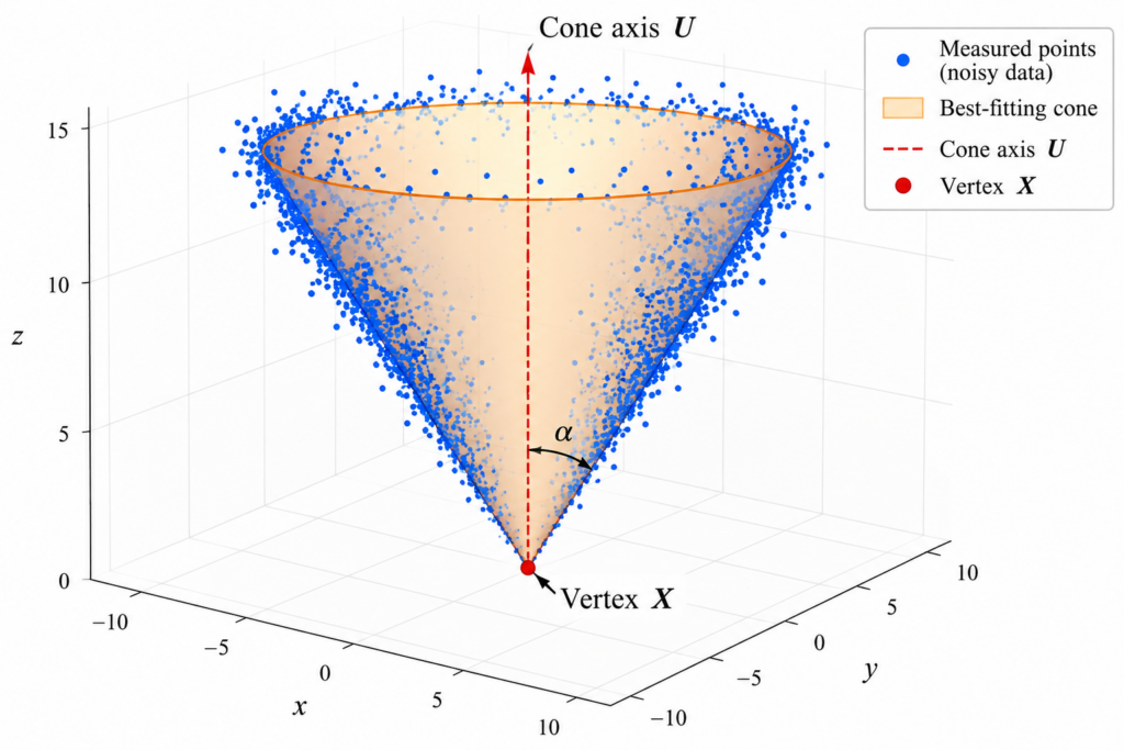
Given thousands of measured points in three-dimensional space, find the cone that best fits them.

But there was an additional requirement that changed the problem completely. The calculation had to be fast enough to be used in real time.

It is one thing to describe an optimization problem mathematically. It is another thing to solve it repeatedly, quickly, and reliably while a real system is operating.

The solution came from combining elementary geometry with nonlinear least squares and the Gauss–Newton method.

The Geometric Problem

Suppose a collection of measured points

$P_{1}, P_{2}, \dots, P_{m}$

lies close to the surface of an unknown right circular cone.

We want to determine three things:

the vertex of the cone, the direction of its axis, and its opening angle.

Let

$X = (x_{1}, x_{2}, x_{3})$

be the vertex, let $U$ point along the axis, and let $α$ be the half-angle of the cone.

If $P$ lies exactly on the cone, then the vector

$P - X$

makes angle $α$ with the cone axis.

The dot-product formula for the angle between two vectors therefore gives

${({(P - X)}^{T} U)}^{2} = {‖ P - X ‖}^{2} {‖ U ‖}^{2} {cos α}^{2} .$

This one equation contains the geometry of the cone.

Turning Geometry into an Error

Measured data will not lie exactly on a perfect cone. There will be noise, measurement error, and small deviations from the ideal surface.

So instead of asking whether a point satisfies the cone equation exactly, we measure how far it is from satisfying the equation.

Define the residual

$R (P) = {‖ P - X ‖}^{2} {cos α}^{2} - \frac{{({(P - X)}^{T} U)}^{2}}{{‖ U ‖}^{2}} .$

For a point exactly on the cone,

$R (P) = 0 .$

For a measured point near the cone, the residual will generally be nonzero.

Why Use This Residual?

There is an important practical point here.

One could try to calculate the exact shortest geometric distance from every measured point to the cone. But when thousands of points must be processed repeatedly in real time, the computational form of the problem matters.

The residual above is obtained directly from the cone equation. It can be evaluated using additions, multiplications, dot products, and a few simple functions.

This was exactly what was needed for the application: a mathematical description that could be differentiated explicitly and evaluated rapidly.

Six Unknown Parameters

The direction of the axis does not depend on the length of $U$ . Multiplying the axis vector by a nonzero constant gives the same axis.

Assuming the axis is not parallel to the $(x_{1}, x_{2})$ plane, we can therefore write

$U = (u_{1}, u_{2}, 1) .$

The entire cone is then described by only six unknown numbers:

$S = {(x_{1}, x_{2}, x_{3}, u_{1}, u_{2}, α)}^{T} .$

Three numbers locate the vertex, two determine the axis direction, and one determines the cone angle.

From One Point to Thousands of Points

Suppose there are $m$ measured points.

For each point $P_{j}$ , compute a residual $R_{j}$ .

We then look for the cone that minimizes the total squared residual:

$f (S) = \frac{1}{2} \sum_{j = 1}^{m} R_{j}^{2} .$

This is a nonlinear least-squares problem.

Why Not Just Solve the Equations?

If the measurements were perfect, six carefully chosen points might appear to be enough to determine six unknown parameters.

Real data do not work that way.

Measurements contain noise, and a small collection of points may give a poor estimate. Instead, we can use hundreds or thousands of points simultaneously and find the cone that best fits all of them.

But now the equations are nonlinear. There is no simple matrix formula that immediately gives the answer.

This is where Gauss–Newton enters the story.

The Jacobian

Put all the residuals into one vector:

$E = {(R_{1}, R_{2}, \dots, R_{m})}^{T} .$

Then

$f = \frac{1}{2} {‖ E ‖}^{2} .$

The Jacobian $J$ contains the derivatives of every residual with respect to the six cone parameters.

Its $j$ -th row is

$J_{j} = (\frac{\partial R_{j}}{\partial x_{1}}, \frac{\partial R_{j}}{\partial x_{2}}, \frac{\partial R_{j}}{\partial x_{3}}, \frac{\partial R_{j}}{\partial u_{1}}, \frac{\partial R_{j}}{\partial u_{2}}, \frac{\partial R_{j}}{\partial α}) .$

In the actual implementation, these derivatives were derived analytically rather than estimated numerically.

That requires more work at the beginning, but once the formulas are known, they can be evaluated very efficiently.

The Key Gauss–Newton Approximation

The gradient of the least-squares objective has a particularly simple form:

$\nabla f = J^{T} E .$

The exact Hessian is

$\nabla^{2} f = J^{T} J + \sum_{j = 1}^{m} R_{j} \nabla^{2} R_{j} .$

Computing the second term repeatedly is considerably more expensive.

Gauss–Newton makes the approximation

$\nabla^{2} f \approx J^{T} J .$

This approximation becomes especially natural when the fit is already good, because the residuals $R_{j}$ are then small.

That observation was crucial for a real-time implementation. Instead of constructing the complete second derivative at every iteration, we can work primarily with the Jacobian.

One Iteration

At the current estimate $S_{k}$ , the Gauss–Newton direction $G_{k}$ is obtained by solving

${J_{k}}^{T} J_{k} G_{k} = - {J_{k}}^{T} E_{k} .$

Then update the six cone parameters:

$S_{k + 1} = S_{k} + a_{k} G_{k} .$

Here $0 < a_{k} \leq 1$ is the step length.

Why Use a Line Search?

Taking the full Gauss–Newton step is not always a good idea when the current estimate is still far from the solution.

The implementation therefore reduces the step when necessary until the objective function decreases sufficiently.

In mathematical form, choose the step length so that

$f (S_{k} + a_{k} G_{k}) \leq f (S_{k}) + ρ a_{k} {\nabla f_{k}}^{T} G_{k} .$

The purpose is simple: do not accept an iteration that moves too aggressively in a direction that fails to improve the fit sufficiently.

The Real-Time Idea

At first glance this may still look like a large calculation. There may be thousands of measured points.

But notice something important.

No matter how many data points we have, there are still only six unknown cone parameters.

The Jacobian may have thousands of rows, but only six columns. The matrix

$J^{T} J$

is therefore only

$6 \times 6 .$

Similarly,

$J^{T} E$

has only six components.

So the data set can be large while the system that must be solved at each Gauss–Newton iteration remains very small.

This is exactly the type of structure one wants to exploit in a real-time numerical algorithm.

Did It Work?

Yes.

This was not an exercise invented to demonstrate Gauss–Newton. I developed the method because the cone-fitting calculation was needed in a real application, and it had to operate in real time.

The implementation worked extremely well.

That experience taught me an important lesson about applied mathematics: the best mathematical formulation is not necessarily the one that looks most sophisticated on paper.

Sometimes the decisive question is:

Can we formulate the problem so that the computer can solve it quickly enough to be useful?

Why the Approximation Works

There is another nice feature of Gauss–Newton.

Recall that the exact Hessian is

$\nabla^{2} f = J^{T} J + \sum_{j = 1}^{m} R_{j} \nabla^{2} R_{j} .$

As the estimated cone approaches the data, the residuals become small. Consequently, the second term becomes less important and

$\nabla^{2} f \approx J^{T} J .$

So as the algorithm approaches a good fit, the inexpensive approximation becomes increasingly appropriate.

A Final Check

Although computing the full Hessian at every iteration is expensive, it can still be useful after the optimization has finished.

At the final solution we can evaluate

$\nabla^{2} f = J^{T} J + \sum_{j = 1}^{m} R_{j} \nabla^{2} R_{j} .$

If its eigenvalues are positive, the Hessian is positive definite and the computed stationary point is a local minimum.

In other words, we use the inexpensive approximation while speed matters, and we can use the more expensive calculation afterward as a check.

The Larger Lesson

The mathematics of this problem can be summarized in one chain:

3D measurements → cone geometry → residuals → least squares → Jacobian → Gauss–Newton → real-time fit.

The cone itself is elementary geometry. Least squares is a classical idea. The derivatives require calculus. Gauss–Newton comes from numerical optimization.

None of these ingredients alone solves the practical problem.

The solution comes from putting them together in a form that a computer can evaluate rapidly.

That is one of the most satisfying aspects of applied mathematics: sometimes a few familiar mathematical ideas, combined in the right way, turn a difficult real-world computation into something that works almost like magic.

A Closely Related Fitting Problem

Fitting a cone to a large cloud of measured points is one example of a broader problem: how can we recover a geometric surface accurately when the computation has to be fast enough for real-time use?

A closely related problem replaces the cone by a cylinder. The geometry changes, but the same practical challenge remains: turn thousands of measurements into a reliable geometric fit without an expensive general-purpose optimization.

Continue exploring: How Do You Fit a Cylinder to Thousands of Points in Real Time?

October 1, 2026

Why Does an OFDM Signal Have a Rayleigh Distribution?

A complicated communication signal can sometimes be understood using surprisingly elementary mathematics.

Consider a large number of vectors of length 1 pointing in random directions. Add them together. What can we say about the length of the resulting vector?

This seemingly geometric probability problem leads directly to a standard mathematical model for OFDM (Orthogonal Frequency-Division Multiplexing), a technique used in modern digital communication.

The path is beautiful:

random phases → sine and cosine → Central Limit Theorem → two-dimensional Gaussian → Rayleigh distribution.

Step 1: Add Random Unit Vectors

Suppose that

θ_{1}, θ_{2}, \dots, θ_{N}

are independent random angles uniformly distributed between 0 and $2 π$ .

The corresponding unit complex numbers are

e^{i θ_{k}} = cos θ_{k} + i sin θ_{k} .

Now add all of them:

Z = \sum_{k = 1}^{N} e^{i θ_{k}} .

Separating the real and imaginary parts gives

Z = X + i Y,

where

X = \sum_{k = 1}^{N} cos θ_{k}, Y = \sum_{k = 1}^{N} sin θ_{k} .

Step 2: What Is the Distribution of One Coordinate?

If $θ$ is uniformly distributed on $[0, 2 π]$ , then both $sin θ$ and $cos θ$ have density

g (x) = \frac{1}{π \sqrt{1 - x^{2}}}, - 1 < x < 1 .

This is sometimes called the arcsine distribution.

By symmetry,

E [cos θ] = E [sin θ] = 0 .

Also,

E [{cos θ}^{2}] = E [{sin θ}^{2}] = \frac{1}{2} .

Therefore each coordinate has mean 0 and variance $\frac{1}{2}$ .

Step 3: The Central Limit Theorem Appears

Now comes the key step.

Both $X$ and $Y$ are sums of many independent random variables.

When $N$ is large, the Central Limit Theorem tells us that these sums are approximately normally distributed:

X \approx N (0, \frac{N}{2}),

Y \approx N (0, \frac{N}{2}) .

In other words, the endpoint of our random walk is approximately described by a two-dimensional Gaussian distribution centered at the origin.

Step 4: How Far Are We from the Origin?

The amplitude of the complex sum is

R = | Z | = \sqrt{X^{2} + Y^{2}} .

So we have reached a purely geometric question:

If a point has two independent Gaussian coordinates, what is the distribution of its distance from the origin?

The answer is the Rayleigh distribution.

Since each coordinate has variance $\frac{N}{2}$ , the approximate density of $R$ is

f (r) \approx \frac{2 r}{N} \exp (- \frac{r^{2}}{N}), r \geq 0 .

This formula is important to interpret correctly. For a finite number of random unit vectors it is generally not the exact distribution. It is the large- $N$ approximation produced by the Central Limit Theorem.

A Shorter Derivation of the Rayleigh Formula

There is also a beautiful geometric way to obtain the density.

For large $N$ , the joint density of $(X, Y)$ is approximately

p (x, y) = \frac{1}{π N} \exp (- \frac{x^{2} + y^{2}}{N}) .

This density depends only on the distance from the origin.

A thin circular ring of radius $r$ and thickness $d r$ has area approximately

2 π r d r .

Multiplying the two-dimensional density by this ring area gives

\frac{1}{π N} \exp (- \frac{r^{2}}{N}) \cdot 2 π r d r .

Therefore,

f (r) = \frac{2 r}{N} \exp (- \frac{r^{2}}{N}) .

So the factor $r$ in the Rayleigh distribution has a simple geometric origin: circles become longer as their radius increases.

What Does This Have to Do with OFDM?

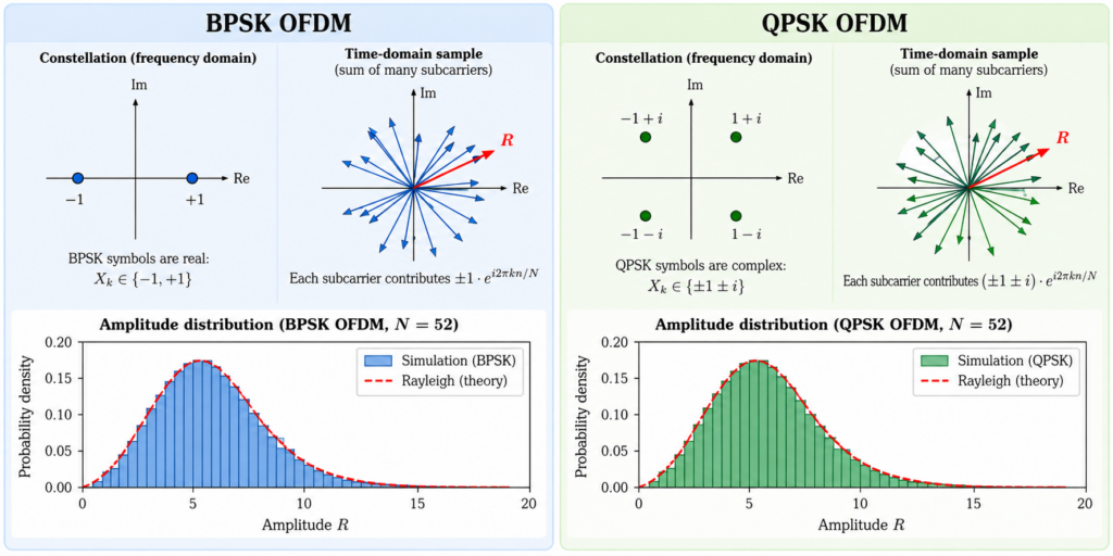
An OFDM time-domain sample is produced by an inverse discrete Fourier transform. It therefore involves adding many complex contributions having different phases.

This suggests viewing the sample, in a simplified model, as a sum of many complex vectors.

That brings us back to exactly the random-vector problem above.

An Example with 52 Active Carriers

Consider a system with 64 available carrier positions, of which 52 are nonzero: 48 data carriers and 4 pilot carriers.

The simple random-phasor model therefore suggests taking

N = 52 .

For a Rayleigh distribution with the density derived above, the expected amplitude is

E [R] = \frac{\sqrt{π N}}{2} .

For $N = 52$ , this gives

E [R] = \frac{\sqrt{52 π}}{2} \approx 6.3907 .

How Good Is the Approximation?

I originally investigated this question numerically by comparing the simple theoretical model with simulated OFDM signals.

The theoretical mean amplitude for the 52-vector model is approximately 6.3907.

A direct simulation of the random-vector model produced 6.3796.

The corresponding simulated OFDM mean amplitudes were:

Model	Mean amplitude
Rayleigh theory	6.3907
Random-vector simulation	6.3796
BPSK OFDM	6.3889
QPSK OFDM	6.4015
16QAM OFDM	6.4058
64QAM OFDM	6.3837

The agreement is remarkably good.

A complicated digital communication signal has, at least at the level of its typical amplitude, been captured by a very simple model: add 52 vectors pointing in random directions.

But What About Rare Peaks?

Matching the average is not the whole story.

For communication systems, unusually large signal peaks are important. An amplifier must be able to accommodate those peaks without severe distortion.

This is where the difference between an approximation and an exact distribution becomes important.

In the original numerical experiment, the simple theory tracked several OFDM simulations quite well at moderate thresholds. But differences appeared in the far tail of the distribution, particularly for BPSK.

For example, at a peak-to-average threshold of 12 dB, the values from that simulation were approximately

Model	Tail probability
Simple theory	4.0 × 10⁻⁶
BPSK	1.969 × 10⁻³
QPSK	9.4 × 10⁻⁵
16QAM	7.9 × 10⁻⁵
64QAM	4.0 × 10⁻⁵

This illustrates an important lesson in probability.

Two distributions can look very similar around their typical values while behaving quite differently in their extreme tails.

The Central Limit Theorem explains the center of the distribution extremely well, but rare events can require more careful analysis.

The Mathematics Behind a Communication Signal

What I like about this example is the number of mathematical ideas that meet in one problem.

We started with complex numbers:

e^{i θ} = cos θ + i sin θ .

Those became random vectors in the plane.

Their coordinates led to probability distributions.

Adding many of them brought in the Central Limit Theorem.

The resulting two-dimensional Gaussian led, through elementary geometry, to the Rayleigh distribution:

f (r) \approx \frac{2 r}{N} \exp (- \frac{r^{2}}{N}) .

And that simple formula gives a surprisingly accurate description of the amplitude of an OFDM signal.

This is a good example of why mathematical modeling is so useful: the real system may be complicated, but sometimes the right simplified model exposes the mathematics underneath it.

Where the Gaussian Function Enters the Story

The Rayleigh distribution in OFDM is closely connected to Gaussian random variables. When many independent contributions combine, the in-phase and quadrature components of the signal are approximately Gaussian, and their magnitude produces the Rayleigh distribution.

At the heart of the Gaussian distribution is the remarkable function $e^{- x^{2}}$ . Its integral over the real line cannot be evaluated by finding an ordinary elementary antiderivative. Yet there is a beautiful way to compute it by moving from one dimension to two.

Continue exploring: The Gaussian Integral and Beyond: From e^(-x²) to a Family of Integrals

October 1, 2026

A Sum of Cosines Is a Geometric Series—Could You Believe It?

Consider the innocent-looking sum

$S = cos x + cos 2 x + cos 3 x + \dots + cos n x .$

At first glance, there is nothing geometric about it. The terms are cosines, not powers of a common ratio.

But there is a geometric series hiding inside.

The Key Idea

Euler’s formula says

$e^{i x} = cos x + i sin x .$

Therefore, the real part of $e^{i k x}$ is $cos k x$ . Hence

$S = Re (e^{i x} + e^{2 i x} + e^{3 i x} + \dots + e^{n i x}) .$

Now look carefully at the expression inside the parentheses. It is a geometric series!

Its first term is $e^{i x}$ , and its common ratio is also $e^{i x}$ .

Sum the Geometric Series

Using the finite geometric-series formula,

$e^{i x} + e^{2 i x} + \dots + e^{n i x} = e^{i x} \frac{1 - e^{n i x}}{1 - e^{i x}} .$

This already proves that our trigonometric sum comes from a geometric series. But we can simplify it further.

A Useful Identity

For any real number $t$ ,

$1 - e^{i t} = - 2 i e^{i t / 2} sin (\frac{t}{2}) .$

Apply this identity to both the numerator and denominator. After cancellation, we obtain

$e^{i x} + e^{2 i x} + \dots + e^{n i x} = \frac{sin (\frac{n x}{2})}{sin (\frac{x}{2})} e^{i \frac{(n + 1) x}{2}} .$

Now take the real part. Since the real part of $e^{i θ}$ is $cos θ$ , we arrive at

$cos x + cos 2 x + \dots + cos n x = \frac{sin (\frac{n x}{2}) cos (\frac{(n + 1) x}{2})}{sin (\frac{x}{2})} .$

So the final formula is

$cos x + cos 2 x + \dots + cos n x = \frac{sin (\frac{n x}{2}) cos (\frac{(n + 1) x}{2})}{sin (\frac{x}{2})} .$

This formula applies whenever $sin (x / 2) \neq 0$ . If $x$ is a multiple of $2 π$ , every cosine equals 1, so the original sum is simply $n$ .

There Is Geometry Behind the Geometric Series

The connection is even more interesting than the algebra suggests.

Each complex number

$e^{i k x} = cos k x + i sin k x$

can be viewed as a vector of length 1 making an angle $k x$ with the positive horizontal axis.

Thus the vectors

$e^{i x}, e^{2 i x}, e^{3 i x}, \dots, e^{n i x}$

all have the same length, and each successive vector is obtained by rotating the previous one through exactly the same angle $x$ .

Place these vectors head-to-tail. They form a turning polygonal chain. Their vector sum is

$e^{i x} + e^{2 i x} + \dots + e^{n i x} .$

And what is the horizontal component of this vector?

Exactly

$cos x + cos 2 x + \dots + cos n x .$

So our sum of cosines really does have a geometric meaning.

And the Sines Come for Free

The imaginary part of exactly the same geometric series gives another classical identity:

$sin x + sin 2 x + \dots + sin n x = \frac{sin (\frac{n x}{2}) sin (\frac{(n + 1) x}{2})}{sin (\frac{x}{2})} .$

One geometric series has given us two trigonometric identities.

The Takeaway

A sum such as

$cos x + cos 2 x + \dots + cos n x$

does not look remotely like a geometric series.

But complex numbers reveal what is hidden:

$trigonometric sum \to complex exponentials \to geometric series \to closed formula.$

Sometimes the hardest part of a problem is not doing the calculation. It is recognizing what the calculation really is.

Another Unexpected Side of Trigonometry

Writing a sum of cosines as part of a geometric series reveals algebra hidden inside trigonometry. There is another beautiful example of this idea in the historical problem of actually computing sines and cosines.

Long before electronic calculators, Newton developed infinite series that turned $\sin (x)$ and $\cos (x)$ into expressions that could be evaluated using arithmetic.

Continue exploring: How Newton Computed Sines and Cosines Without a Calculator

October 1, 2026
Can a Curve Fill a Square? The Mathematics of Space-Filling Curves

Can a Curve Fill a Square?

A curve is one-dimensional. A square is two-dimensional. So it seems impossible that a single continuous curve could pass through every point of a square.

Surprisingly, it can.

There exists a continuous function
$H : [0, 1] \to [0, 1] \times [0, 1]$
whose image is the entire unit square. In other words, as the parameter moves continuously from 0 to 1, the point $H (t)$ eventually reaches every point of the square.

Such a curve is called a space-filling curve.

The Hilbert Curve

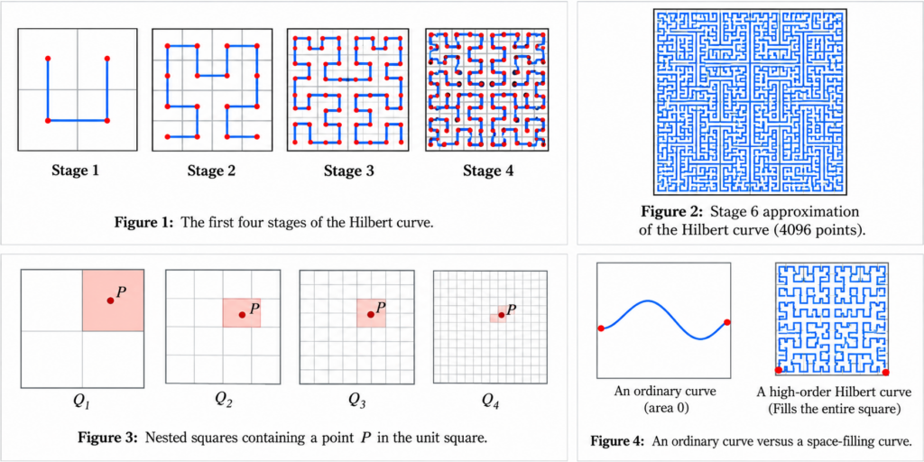
One of the most beautiful examples is the Hilbert curve. Instead of trying to draw the final curve immediately, we construct a sequence of increasingly complicated polygonal curves.

Start with a square. Divide it into four equal smaller squares and connect their centers in an order that forms a U-shaped path.

This is the first approximation.

For the second approximation, divide each of the four squares into four smaller squares. We now have
$4^{2} = 16$
small squares. Inside each group of four, place a suitably rotated or reflected copy of the previous pattern and connect the pieces.

Repeat the process again and again.

At stage $n$ , the square has been divided into
$4^{n}$
small squares, each having side length
$2^{- n} .$
The Squares Become Tiny

The important feature of the construction is not merely that the number of squares increases. Their size simultaneously decreases to zero.

A small square at stage $n$ has side length
$\frac{1}{2^{n}},$
so its diameter is
$\frac{\sqrt{2}}{2^{n}} .$
Therefore,
$\frac{\sqrt{2}}{2^{n}} \to 0 as n \to \infty .$
The construction is examining the square on smaller and smaller scales.

Why Does the Limit Fill the Square?

Take any point $P$ in the unit square.

At the first stage, $P$ belongs to at least one of the four small squares. Call one such square $Q_{1}$ .

At the second stage, choose one of the smaller squares containing $P$ and call it $Q_{2}$ . Continue in this way.

We obtain nested squares
$Q_{1} \supseteq Q_{2} \supseteq Q_{3} \supseteq \dots$
containing $P$ , while
$diam (Q_{n}) \to 0 .$
Since the squares shrink to a point, their intersection is precisely
$⋂_{n = 1}^{\infty} Q_{n} = {P} .$
The Hilbert construction assigns corresponding nested parameter intervals
$I_{1} \supseteq I_{2} \supseteq I_{3} \supseteq \dots$
whose lengths also tend to zero. Their intersection therefore determines a parameter value $t$ . For this value,
$H (t) = P .$
But $P$ was an arbitrary point of the square. Thus the limiting curve reaches every point of the square.

A Curve Whose Image Has Area 1

This produces a remarkable conclusion.

The domain of the Hilbert curve is the interval $[0, 1]$ , but its image is
$H ([0, 1]) = [0, 1] \times [0, 1] .$
Consequently, the image of this continuous curve has area
$1 .$
This is very different from an ordinary smooth curve, whose area in the plane is zero.

What Happens to the Length?

The polygonal approximations also reveal something interesting.

At stage $n$ , the curve visits $4^{n}$ small squares. The characteristic distance between neighboring points is of order
$2^{- n} .$
Therefore the total length is of order
$4^{n} \cdot 2^{- n} = 2^{n} .$
As $n \to \infty$ , this quantity tends to infinity.
$2^{n} \to \infty .$
Thus the approximations stay inside a square of area 1, but their lengths grow without bound.

Does This Mean an Interval and a Square Are the Same?

No.

The Hilbert curve is continuous and onto, but it is not one-to-one. Different parameter values can correspond to the same point of the square.

This distinction is essential. There is no continuous one-to-one correspondence with a continuous inverse between an interval and a square.

The space-filling curve does something subtler: it continuously folds an interval over itself infinitely many times until its image covers the entire square.

A Dimensional Clue

There is another way to see why the numbers in the construction fit together so naturally.

When lengths are reduced by a factor of 2, the number of pieces increases by a factor of 4:
$4 = 2^{2} .$
If we informally ask for a dimension $d$ satisfying
$4 = 2^{d},$
then
$d = \frac{\log 4}{\log 2} = 2 .$
This scaling behavior gives a hint of how a construction beginning with a one-dimensional parameter can produce an image that occupies a two-dimensional region.

Why Space-Filling Curves Are Useful

Space-filling curves are not only mathematical curiosities. Hilbert-type orderings are useful whenever multidimensional data must be arranged in a one-dimensional sequence.

The Hilbert ordering has an important locality property: points that are close along the curve tend to remain relatively close in space. This idea appears in spatial indexing, image processing, databases, and algorithms for organizing multidimensional data.

A construction that originally seemed almost paradoxical therefore connects pure mathematics with practical computation.

The Main Idea

The Hilbert curve demonstrates how misleading our finite-dimensional intuition can be when a limiting process is repeated infinitely many times.

Every finite approximation is just an ordinary polygonal curve. None of these approximations fills the square.

But the subdivisions become arbitrarily small, and in the limit every point of the square is reached.

A continuous image of a one-dimensional interval can therefore fill an entire two-dimensional square.

Continue exploring: Another surprising example of how strange continuous functions can be: Can a Function Be Continuous Everywhere but Differentiable Nowhere?

Not all interesting curves are as unusual as space-filling curves. Some are designed to create smooth, controllable shapes using only a few points. Discover how this works in Bézier Curves: How Four Points Create Beautiful Shapes .

September 30, 2026
A Surprising Improper Integral: Why the Integral of sin(ax)/x Is Always π/2

A Surprising Improper Integral

Consider the improper integral
$\int_{0}^{\infty} \frac{\sin (a x)}{x} d x .$
At first glance, this integral looks difficult. The factor $\frac{1}{x}$ suggests a singularity at the origin, while the sine function continues to oscillate forever as $x \to \infty$ . There is no elementary antiderivative that immediately resolves the problem.

Nevertheless, for every positive number $a$ , the answer is remarkably simple:
$\int_{0}^{\infty} \frac{\sin (a x)}{x} d x = \frac{π}{2} .$
Even more surprisingly, the answer does not depend on the positive value of $a$ . Let us see why.

The Main Idea: Add a Damping Factor

Instead of attacking the original integral directly, introduce a positive parameter $t$ and define
$F (t) = \int_{0}^{\infty} e^{- t x} \frac{\sin (a x)}{x} d x, t > 0 .$
The factor $e^{- t x}$ suppresses the oscillations for large values of $x$ . This makes the parameter-dependent integral easier to work with.

The key step is to differentiate with respect to the parameter $t$ . We obtain
$F^{'} (t) = - \int_{0}^{\infty} e^{- t x} \sin (a x) d x .$
Notice what happened: the troublesome factor $\frac{1}{x}$ has disappeared. We are left with a standard Laplace-type integral.

Evaluating the Easier Integral

For $t > 0$ , we have
$\int_{0}^{\infty} e^{- t x} \sin (a x) d x = \frac{a}{t^{2} + a^{2}} .$
Therefore,
$F^{'} (t) = - \frac{a}{t^{2} + a^{2}} .$
Now the problem has been reduced to an elementary integral.

Recovering F(t)

As $t \to \infty$ , the exponential damping becomes stronger and
$F (t) \to 0 .$
Thus, for $a > 0$ ,
$F (t) = \int_{t}^{\infty} \frac{a}{u^{2} + a^{2}} d u .$
Evaluating this integral gives
$F (t) = \frac{π}{2} - \arctan (\frac{t}{a}) .$
Equivalently, using the elementary arctangent identity,
$F (t) = \arctan (\frac{a}{t}) .$
So we have actually obtained the more general and useful formula
$\int_{0}^{\infty} e^{- t x} \frac{\sin (a x)}{x} d x = \arctan (\frac{a}{t}), a > 0, t > 0 .$
Removing the Damping

We introduced the exponential factor only to make the integral easier to evaluate. Now let $t \to 0^{+}$ . Then
$\arctan (\frac{a}{t}) \to \frac{π}{2} .$
and the damping factor approaches $1$ . This leads to the celebrated Dirichlet integral
$\int_{0}^{\infty} \frac{\sin (a x)}{x} d x = \frac{π}{2}, a > 0 .$
Why Does the Answer Not Depend on a?

There is also a simple scaling argument that explains why the answer must be the same for every positive $a$ . Set
$u = a x .$
Then
$x = \frac{u}{a}, d x = \frac{d u}{a} .$
Therefore,
$\int_{0}^{\infty} \frac{\sin (a x)}{x} d x = \int_{0}^{\infty} \frac{\sin (u)}{u} d u .$
The parameter $a$ has completely disappeared. Changing $a$ changes how rapidly the sine function oscillates, but the total value of the improper integral remains unchanged.

What If a Is Zero or Negative?

If $a = 0$ , the integrand is identically zero, so the integral is zero.

If $a < 0$ , use the oddness of the sine function:
$\sin (a x) = - \sin (- a x) .$
Hence the complete result is
$\int_{0}^{\infty} \frac{\sin (a x)}{x} d x = \{\begin{cases} \frac{π}{2} & if a > 0, \\ 0 & if a = 0, \\ - \frac{π}{2} & if a < 0 . \end{cases}$
One Important Detail: The Integral Is Not Absolutely Convergent

The convergence of this integral is subtle. Although
$\int_{0}^{\infty} \frac{\sin (a x)}{x} d x$
converges for $a \neq 0$ , the corresponding absolute-value integral
$\int_{0}^{\infty} \frac{| \sin (a x) |}{x} d x$
diverges. Thus the positive and negative oscillations of the sine function are essential. They cancel one another just enough for the original improper integral to converge.

A Useful Lesson

The most interesting part of this calculation is not simply the final answer $\frac{π}{2}$ . It is the method.

When an integral is difficult to evaluate directly, it can sometimes be embedded into a family of integrals depending on a parameter. Differentiating with respect to that parameter may transform the original problem into a much easier one. After solving the parameterized problem, we return to the original integral by taking a limit.

In this example, the chain of ideas is
$\frac{\sin (a x)}{x} \to e^{- t x} \frac{\sin (a x)}{x} \to F^{'} (t) \to F (t) \to \frac{π}{2} .$
A difficult oscillatory improper integral has been reduced to an elementary rational integral. That is what makes the Dirichlet integral such a beautiful example of the power of introducing a parameter.

Another Surprise from an Improper Integral

The integral involving $\frac{\sin (a x)}{x}$ shows that an oscillating function extending over an infinite interval can nevertheless produce a beautifully simple finite value.

There is another famous improper-integral paradox in which infinity appears in a completely different way: a surface extending forever can enclose a finite volume while having infinite surface area.

Continue exploring: Gabriel’s Horn: When Can an Infinite Horn Be Painted?

From the Dirichlet Integral to the Gaussian Integral

There is another beautiful connection behind the Dirichlet integral. The Gaussian function $e^{- x^{2}}$ leads to one of the most famous improper integrals in mathematics. Its evaluation introduces a remarkably powerful idea: turn a one-dimensional integral into a two-dimensional one and then use geometry.

That same Gaussian structure appears in many unexpected places and provides another route into the world of remarkable improper integrals.

Continue exploring: The Gaussian Integral and Beyond: From e^(-x²) to a Family of Integrals

September 29, 2026

Can a Circle Centered Outside Another Circle Cut Its Area Exactly in Half?

Choose any point outside a circle. Can we draw a second circle, centered at that point, that covers exactly half the area of the original circle?

Surprisingly, the answer is always yes. Even better, there is exactly one such circle.

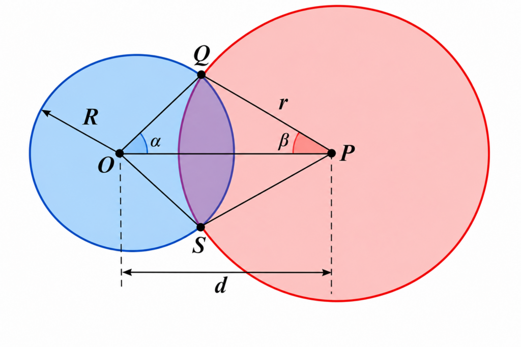
Let the original circle have center O and radius R. Choose a fixed point P outside the circle, and let

d = O P > R .

We want to find the radius r of a circle centered at P that covers exactly half of the original disk.

Why must such a circle exist?

Before calculating anything, we can prove that the desired circle must exist.

Let A(r) denote the area of the part of the original disk covered by the circle centered at P with radius r.

Since P is outside the original circle, the distance from P to the nearest point of the original circle is

d - R .

Therefore, when

r = d - R,

the two circles are externally tangent. They meet at only one point, so their common area is zero:

A (d - R) = 0 .

Now continue increasing r. Eventually,

r = d + R .

At this point the circle centered at P contains the entire original disk. Hence

A (d + R) = π R^{2} .

As r increases, the circle centered at P grows continuously. Consequently, the area A(r) that it covers inside the original circle also changes continuously.

It starts at

0

and eventually reaches

π R^{2} .

Therefore, by the Intermediate Value Theorem, at some intermediate radius it must equal

\frac{1}{2} π R^{2} .

Thus there is at least one radius satisfying

d - R < r < d + R

for which the second circle covers exactly half of the original disk.

Why is the radius unique?

Suppose

r_{1} < r_{2} .

The disk centered at P with the smaller radius is strictly contained in the disk with the larger radius. While the two circles intersect, increasing the radius captures an additional region of positive area inside the original disk.

Therefore A(r) is strictly increasing for

d - R < r < d + R .

So the value

A (r) = \frac{1}{2} π R^{2}

can occur only once. The required circle is therefore unique.

Now let us calculate its radius

Let the two circles intersect at points Q and S. Consider the triangle formed by O, P, and Q.

Its side lengths are

O Q = R, P Q = r, O P = d .

Let α be the angle at O between OP and OQ, and let β be the angle at P between PO and PQ.

By the Law of Cosines,

\cos α = \frac{d^{2} + R^{2} - r^{2}}{2 d R} .

Hence

α = \arccos (\frac{d^{2} + R^{2} - r^{2}}{2 d R}) .

Applying the Law of Cosines at P gives

\cos β = \frac{d^{2} + r^{2} - R^{2}}{2 d r},

β = \arccos (\frac{d^{2} + r^{2} - R^{2}}{2 d r}) .

The area of the overlap

The common lens consists of two circular segments.

At O, the full central angle subtending the common chord is 2α. The area of the corresponding sector is

R^{2} α .

The triangle inside this sector has area

R^{2} \sin α \cos α .

Thus the first circular segment has area

R^{2} (α - \sin α \cos α) .

Similarly, the second circular segment has area

r^{2} (β - \sin β \cos β) .

Therefore the total overlap area is

A (r) = R^{2} (α - \sin α \cos α) + r^{2} (β - \sin β \cos β) .

The equation for the radius

We want the overlap to be exactly half the area of the original circle. Therefore r must satisfy

R^{2} (α - \sin α \cos α) + r^{2} (β - \sin β \cos β) = \frac{1}{2} π R^{2},

where

α = \arccos (\frac{d^{2} + R^{2} - r^{2}}{2 d R})

and

β = \arccos (\frac{d^{2} + r^{2} - R^{2}}{2 d r}) .

This is a transcendental equation, so in general the radius is found numerically. But our geometric argument has already established something important: for every d > R, this equation has exactly one solution in

d - R < r < d + R .

A scale-free version

The problem really depends only on the ratio d/R. Define

D = \frac{d}{R}, ρ = \frac{r}{R} .

Then D > 1, and the required value of ρ depends only on D. Once ρ is found, the actual radius is simply

r = ρ R .

For example, if the outside point happens to satisfy

d = 2 R,

the numerical solution is

r \approx 2.08225 R .

But this is only one example. The construction works for every point outside the original circle.

The geometric conclusion

We have proved the following result:

Given any point outside a circle, there exists a unique circle centered at that point whose intersection with the original disk has exactly half the area of the original disk.

The calculation of its radius requires solving a transcendental equation, but its existence does not. It follows from a simple geometric idea: start with a circle that barely touches the original circle and continuously increase its radius. The covered area grows continuously from zero to the entire area of the original disk, and therefore it must pass through exactly one-half.

Some numerical examples

Because the problem is unchanged by scaling, we may take

R = 1 .

For several choices of the distance d from the center of the original circle to the outside point, the table below gives the unique radius r that covers exactly half of the original disk.

Distance d	Required radius r
1.10	1.24543
1.25	1.37910
1.50	1.60860
2.00	2.08225
2.50	2.56611
3.00	3.05523
5.00	5.03326

For a circle of arbitrary radius R, these numbers should be interpreted as ratios. For example,

\frac{d}{R} = 2

gives

\frac{r}{R} \approx 2.08225,

or equivalently,

r \approx 2.08225 R .

The table also reveals an interesting pattern: as the outside point moves farther from the original circle, the required radius becomes increasingly close to the distance d itself.

Another Equal-Area Problem

Dividing the area of a circle exactly in half with another circle raises a natural geometric question: can a circle do the same thing to a triangle?

Continue exploring: Can a Circle Cut a Triangle in Half?

September 28, 2026

How Newton Computed Sines and Cosines Without a Calculator

Today, if we want to know the sine or cosine of an angle, we simply press a button on a calculator. But suppose there is no calculator, no computer, and no trigonometric table.

How could we actually compute, for example,
$\sin (1 °)$
using only arithmetic?

One answer comes from the classical sine and cosine series associated with Isaac Newton. The series appeared in Newton’s De analysi per aequationes numero terminorum infinitas, written in 1665–1666. The elegant derivation below follows a later mean-value approach presented by Heinrich Dörrie, written here in modern calculus notation.

The goal

We want formulas that allow us to calculate the sine and cosine of an angle x. The angle must be measured in radians.

The formulas we will obtain are
$\sin x = x - \frac{x^{3}}{3!} + \frac{x^{5}}{5!} - \frac{x^{7}}{7!} + \dots$
and
$\cos x = 1 - \frac{x^{2}}{2!} + \frac{x^{4}}{4!} - \frac{x^{6}}{6!} + \dots$
Today these are familiar power series. What is especially interesting is that we can derive them from a very simple idea: repeatedly taking averages.

The key idea: average values

Consider the average value of the sine function on the interval from 0 to x. In modern calculus notation,
$\frac{1}{x} \int_{0}^{x} \sin t d t = \frac{1 - \cos x}{x}$
Similarly, the average value of cosine is
$\frac{1}{x} \int_{0}^{x} \cos t d t = \frac{\sin x}{x}$
These two elementary formulas are enough to generate increasingly accurate approximations for both sine and cosine.

Start with the simplest inequality

For a positive angle x sufficiently close to zero,
$\cos x < 1$
Now take the average of both sides from 0 to x. The average of the left side is
$\frac{\sin x}{x}$
while the average of 1 is simply 1. Therefore,
$\frac{\sin x}{x} < 1$
and hence
$\sin x < x$
We have obtained our first approximation:
$\sin x \approx x$
Average again

Now start with
$\sin x < x$
and take averages once more. The average of the left side is
$\frac{1 - \cos x}{x}$
while the average of the function t on the interval from 0 to x is x/2. Thus,
$\frac{1 - \cos x}{x} < \frac{x}{2}$
Multiplying by x and rearranging gives
$\cos x > 1 - \frac{x^{2}}{2!}$
And again

Take averages of this new inequality. The average of cosine is
$\frac{\sin x}{x}$
and the average of the right-hand side is
$1 - \frac{x^{2}}{6}$
Therefore,
$\frac{\sin x}{x} > 1 - \frac{x^{2}}{6}$
and consequently
$\sin x > x - \frac{x^{3}}{3!}$
We have now trapped sine between two simple expressions:
$x - \frac{x^{3}}{3!} < \sin x < x$
Keep repeating the process

Each time we take another average, we obtain another term. Continuing gives alternating upper and lower bounds:
$\sin x < x - \frac{x^{3}}{3!} + \frac{x^{5}}{5!}$
and then
$\sin x > x - \frac{x^{3}}{3!} + \frac{x^{5}}{5!} - \frac{x^{7}}{7!}$
The upper and lower approximations become closer and closer. Their common limiting value gives
$\sin x = x - \frac{x^{3}}{3!} + \frac{x^{5}}{5!} - \frac{x^{7}}{7!} + \dots$
The same procedure gives
$\cos x = 1 - \frac{x^{2}}{2!} + \frac{x^{4}}{4!} - \frac{x^{6}}{6!} + \dots$
A built-in error estimate

There is another important advantage. If we stop either series after a finite number of terms, the error is smaller in absolute value than the first term we leave out.

For example, if we use
$\sin x \approx x - \frac{x^{3}}{3!}$
then the error is smaller than
$\frac{x^{5}}{5!}$
This means that the series does not merely give us an approximation. It also tells us how accurate that approximation is.

Computing sin(1°)

Now let us actually calculate a trigonometric value without using a table.

One degree in radians is
$x = \frac{π}{180} \approx 0.01745329252$
Since this number is very small, just two terms of the sine series already give extraordinary accuracy:
$\sin (1 °) \approx x - \frac{x^{3}}{6}$
Substituting the value of x gives
$\sin (1 °) \approx 0.0174524064$
How accurate is this?

The first omitted term is
$\frac{x^{5}}{120} < 0.00000000002$
Thus only two terms are enough to determine sin(1°) correctly to ten decimal places:
$\sin (1 °) \approx 0.0174524064$
That is a remarkable amount of accuracy from such a short calculation.

Computing the cosine

The cosine works in exactly the same way. For one degree,
$\cos x \approx 1 - \frac{x^{2}}{2} + \frac{x^{4}}{24}$
which gives
$\cos (1 °) \approx 0.9998476952$
Again, only a few arithmetic operations are needed.

Why radians matter

There is one essential detail: these formulas require angles to be measured in radians.

The fundamental approximation
$\sin x \approx x$
works in this form because radian measure connects an angle directly with arc length on the unit circle.

If an angle is given in degrees, convert it first:
$x = (angle in degrees) \frac{π}{180}$
The larger idea

What makes this argument beautiful is not merely the final formulas. It is how little we need in order to discover them.

We begin with the elementary inequality
$\cos x < 1$
and repeatedly take average values. Each step produces another power of x, another factorial in the denominator, and a sharper approximation.

Eventually the familiar patterns emerge:
$\sin x = x - \frac{x^{3}}{3!} + \frac{x^{5}}{5!} - \dots$ $\cos x = 1 - \frac{x^{2}}{2!} + \frac{x^{4}}{4!} - \dots$
A calculator evaluates sine and cosine instantly. These series reveal some of the mathematics behind that computation: trigonometric values can be constructed, digit by digit, using powers, factorials, addition, subtraction, multiplication, and division.

Reference

The mean-value derivation in this article is adapted, using modern calculus notation, from Heinrich Dörrie, 100 Great Problems of Elementary Mathematics: Their History and Solution, translated by David Antin, Dover Publications, Problem 15, “Newton’s Sine and Cosine Series,” pp. 59–63.

Another Unexpected Side of Trigonometry

Newton’s approach shows that familiar trigonometric functions can be reconstructed from infinite algebraic expansions. But there is another surprising algebraic connection hiding in trigonometry.

Consider the finite sum $\cos (x) + \cos (2 x) + \dots + \cos (n x) .$ At first glance, it has nothing to do with a geometric series. Yet a simple change of viewpoint reveals exactly that structure.

Continue exploring: A Sum of Cosines Is a Geometric Series—Could You Believe It?

September 28, 2026
Proving 1 + 1/4 + 1/9 + ⋯ = π²/6 with a Double Integral

One of the most famous identities in mathematics is
$1 + \frac{1}{4} + \frac{1}{9} + \frac{1}{16} + \dots = \frac{π^{2}}{6} .$
In summation notation,
$\sum_{n = 1}^{\infty} \frac{1}{n^{2}} = \frac{π^{2}}{6} .$
This is known as the Basel problem. Euler famously solved it in the eighteenth century. There are many proofs, but one particularly beautiful approach uses a double integral and an unexpected change of variables.

Start with the odd terms

Instead of attacking the entire series immediately, consider only the reciprocals of the odd squares:
$S = 1 + \frac{1}{3^{2}} + \frac{1}{5^{2}} + \frac{1}{7^{2}} + \dots .$
We will first prove that
$S = \frac{π^{2}}{8} .$
The full Basel sum will then follow almost immediately.

Turn the series into a double integral

Consider
$I = \int_{0}^{1} \int_{0}^{1} \frac{1}{1 - x^{2} y^{2}} d x d y .$
For points inside the unit square, the geometric-series identity gives
$\frac{1}{1 - x^{2} y^{2}} = \sum_{n = 0}^{\infty} {x y}^{2 n} .$
Therefore,
$I = \sum_{n = 0}^{\infty} (\int_{0}^{1} x^{2 n} d x) (\int_{0}^{1} y^{2 n} d y) .$
Each one-dimensional integral is
$\int_{0}^{1} x^{2 n} d x = \frac{1}{2 n + 1} .$
Hence
$I = \sum_{n = 0}^{\infty} \frac{1}{{(2 n + 1)}^{2}} .$
Thus the double integral is exactly the sum of the reciprocals of the odd squares:
$I = 1 + \frac{1}{3^{2}} + \frac{1}{5^{2}} + \dots .$
The key change of variables

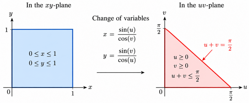
Now comes the surprising part. Introduce new variables u and v by
$x = \frac{\sin (u)}{\cos (v)}, y = \frac{\sin (v)}{\cos (u)} .$
The square
$0 \leq x \leq 1, 0 \leq y \leq 1$
corresponds to the triangular region
$u \geq 0, v \geq 0, u + v \leq \frac{π}{2} .$
To see where the last boundary comes from, notice that
$x \leq 1 \Leftrightarrow \sin (u) \leq \cos (v) \Leftrightarrow u + v \leq \frac{π}{2},$
and the condition on y gives the same inequality.

The Jacobian

We compute
$\frac{\partial x}{\partial u} = \frac{\cos (u)}{\cos (v)}, \frac{\partial x}{\partial v} = \frac{\sin (u) \sin (v)}{{\cos (v)}^{2}} .$
Similarly,
$\frac{\partial y}{\partial u} = \frac{\sin (u) \sin (v)}{{\cos (u)}^{2}}, \frac{\partial y}{\partial v} = \frac{\cos (v)}{\cos (u)} .$
After simplifying the determinant, the Jacobian is
$\frac{\partial (x, y)}{\partial (u, v)} = 1 - x^{2} y^{2} .$
This is exactly the expression that appears in the denominator of our original integral. Therefore,
$\frac{d x d y}{1 - x^{2} y^{2}} = d u d v .$
The complicated-looking integrand has completely disappeared.

The integral becomes an area

Our double integral is now simply
$I = \int_{0}^{\frac{π}{2}} \int_{0}^{\frac{π}{2} - u} d v d u .$
Geometrically, this is the area of a right triangle whose two perpendicular sides both have length
$\frac{π}{2}$
Therefore,
$I = \frac{1}{2} \cdot \frac{π}{2} \cdot \frac{π}{2} = \frac{π^{2}}{8} .$
We have proved that
$1 + \frac{1}{3^{2}} + \frac{1}{5^{2}} + \frac{1}{7^{2}} + \dots = \frac{π^{2}}{8} .$
Recovering the full series

Let
$T = \sum_{n = 1}^{\infty} \frac{1}{n^{2}} .$
Split the series into its odd and even terms. The odd terms have sum
$\frac{π^{2}}{8}$
while the even terms have sum
$\frac{1}{2^{2}} + \frac{1}{4^{2}} + \frac{1}{6^{2}} + \dots = \frac{1}{4} T .$
Consequently,
$T = \frac{π^{2}}{8} + \frac{1}{4} T .$
Thus,
$\frac{3}{4} T = \frac{π^{2}}{8},$
and finally,
$T = \frac{π^{2}}{6} .$
Why this proof is remarkable

We started with an infinite series involving nothing but reciprocals of squares. We then represented part of that series by a double integral over a square. A carefully chosen trigonometric change of variables transformed the square into a triangle and, at the same time, made the integrand disappear.

The infinite series was therefore reduced to the area of a triangle:
$\frac{1}{2} \cdot \frac{π}{2} \cdot \frac{π}{2} = \frac{π^{2}}{8} .$
From there, separating the odd and even terms gives the celebrated result
$\sum_{n = 1} \frac{1}{n^{2}} = \frac{π^{2}}{6} .$
It is a striking example of how an infinite series, a double integral, a trigonometric substitution, and a simple geometric area can all describe the same number.

Another Problem Where Two Dimensions Help

The double-integral proof of the Basel sum illustrates a powerful mathematical idea: sometimes a problem becomes easier when we move to a higher dimension.

One of the most beautiful examples is the Gaussian integral. A one-dimensional integral that resists ordinary antiderivative methods becomes accessible after it is squared and transformed into a two-dimensional integral.

Continue exploring: The Gaussian Integral and Beyond: From e^(-x²) to a Family of Integrals

Long before Euler solved the Basel problem, ancient Greek mathematicians had developed ingenious geometric methods for evaluating infinite sums. In particular, Archimedes used areas of triangles to establish a remarkable infinite series identity. Discover his method in How the Ancient Greeks Summed Infinite Series Without Calculus .

September 28, 2026

Author: anatoly

1. The Simplest Population Model

2. Introducing a Carrying Capacity

We Can Predict the Solutions Without Solving the Equation

Where Is the Population Growing Fastest?

3. Now Let Us Solve the Logistic Equation

4. Was Our Original Equation Really So Bad?

5. Continuous Compound Interest

6. Radioactive Decay

7. One Equation, Many Processes

The Geometry of a Cylinder

Distance from a Point to the Axis

Turning the Geometry into a Residual

Reducing the Number of Unknowns

From Geometry to Least Squares

Why the Derivatives Matter

The Jacobian

Gauss–Newton

Why Thousands of Points Are Not as Bad as They Sound

Do Not Always Take the Full Step

When Do We Stop?

Did It Work?

From Cylinders to Cones

The Larger Lesson

A Closely Related Fitting Problem

The Geometric Problem

Turning Geometry into an Error

Why Use This Residual?

Six Unknown Parameters

From One Point to Thousands of Points

Why Not Just Solve the Equations?

The Jacobian

The Key Gauss–Newton Approximation

One Iteration

Why Use a Line Search?

The Real-Time Idea

Did It Work?

Why the Approximation Works

A Final Check

The Larger Lesson

A Closely Related Fitting Problem

Step 1: Add Random Unit Vectors

Step 2: What Is the Distribution of One Coordinate?

Step 3: The Central Limit Theorem Appears

Step 4: How Far Are We from the Origin?

A Shorter Derivation of the Rayleigh Formula

What Does This Have to Do with OFDM?

An Example with 52 Active Carriers

How Good Is the Approximation?

But What About Rare Peaks?

The Mathematics Behind a Communication Signal

Where the Gaussian Function Enters the Story

The Key Idea

Sum the Geometric Series

A Useful Identity

There Is Geometry Behind the Geometric Series

And the Sines Come for Free

The Takeaway

Another Unexpected Side of Trigonometry

Can a Curve Fill a Square?

The Hilbert Curve

The Squares Become Tiny

Why Does the Limit Fill the Square?

A Curve Whose Image Has Area 1

What Happens to the Length?

Does This Mean an Interval and a Square Are the Same?

A Dimensional Clue

Why Space-Filling Curves Are Useful

The Main Idea

A Surprising Improper Integral

The Main Idea: Add a Damping Factor

Evaluating the Easier Integral

Recovering F(t)

Removing the Damping

Why Does the Answer Not Depend on a?

What If a Is Zero or Negative?

One Important Detail: The Integral Is Not Absolutely Convergent

A Useful Lesson

Another Surprise from an Improper Integral

From the Dirichlet Integral to the Gaussian Integral