Elite Math Program

Tag: optimization

How Do You Fit a Cylinder to Thousands of Points in Real Time?

Several years ago, I was given a practical geometry problem:

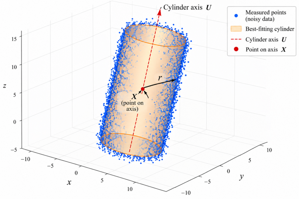
Given thousands of measured points in three-dimensional space, find the cylinder that best fits them.

There was an additional requirement that made the problem much more interesting. The calculation had to be fast enough to operate in real time.

This meant that simply defining a mathematically reasonable fitting problem was not enough. The equations had to be arranged so that thousands of data points could be processed efficiently, the derivatives could be evaluated quickly, and each optimization step would require solving only a very small system of equations.

The resulting method combines geometry, calculus, least squares, and the Gauss–Newton method.

The Geometry of a Cylinder

Suppose that

$X = {(x_{1}, x_{2}, x_{3})}^{T}$

is a point on the axis of a cylinder, and

$U = {(u_{1}, u_{2}, u_{3})}^{T}$

is a vector pointing along the axis.

Let $P$ be a point on the surface of the cylinder.

The defining geometric property is simple:

The perpendicular distance from every point on the cylinder to its axis is the radius $r$ .

Distance from a Point to the Axis

Consider the vector

$P - X .$

Part of this vector points along the cylinder axis, while the remaining part is perpendicular to the axis.

If $α$ is the angle between $P - X$ and $U$ , then

$‖ P - X ‖ sin α = r .$

Squaring gives

${‖ P - X ‖}^{2} {sin α}^{2} = r^{2} .$

The dot product gives

${({(P - X)}^{T} U)}^{2} = {‖ P - X ‖}^{2} {‖ U ‖}^{2} {cos α}^{2} .$

Combining these relations eliminates the angle completely and gives

${‖ P - X ‖}^{2} - \frac{{({(P - X)}^{T} U)}^{2}}{{‖ U ‖}^{2}} = r^{2} .$

This is the equation we need.

The first term measures the squared distance from $X$ to $P$ . The fraction subtracts the squared component parallel to the axis. What remains is exactly the squared perpendicular distance to the axis.

Turning the Geometry into a Residual

Measured points will not lie exactly on a perfect cylinder.

For a measured point $P$ , define

$R (P) = {‖ P - X ‖}^{2} - \frac{{({(P - X)}^{T} U)}^{2}}{{‖ U ‖}^{2}} - r^{2} .$

For a point exactly on the cylinder,

$R (P) = 0 .$

For a noisy measured point, the residual will usually be nonzero.

Reducing the Number of Unknowns

At first the cylinder appears to have seven parameters: three coordinates for a point on its axis, three coordinates for the axis direction, and the radius.

But there is redundancy.

Moving the reference point $X$ along the axis does not change the cylinder. Also, multiplying $U$ by a nonzero constant does not change its direction.

Assuming the cylinder axis is not parallel to the $(x_{1}, x_{2})$ plane, choose

$X = {(x_{1}, x_{2}, 0)}^{T}, U = {(u_{1}, u_{2}, 1)}^{T} .$

Now the entire cylinder is described by only five unknown numbers:

$S = {(x_{1}, x_{2}, u_{1}, u_{2}, r)}^{T} .$

Two numbers locate the axis, two determine its direction, and one gives the radius.

From Geometry to Least Squares

Suppose our measuring system produces $m$ points:

$P_{1}, P_{2}, \dots, P_{m} .$

Each point produces a residual $R_{j}$ .

We find the best-fitting cylinder by minimizing

$f (S) = \frac{1}{2} \sum_{j = 1}^{m} R_{j}^{2} .$

This is a nonlinear least-squares problem.

Why the Derivatives Matter

Because the calculation had to run quickly, I derived the residual derivatives analytically.

For each measured point, we need derivatives with respect to the five unknown parameters:

$\nabla R = (\frac{\partial R}{\partial x_{1}}, \frac{\partial R}{\partial x_{2}}, \frac{\partial R}{\partial u_{1}}, \frac{\partial R}{\partial u_{2}}, \frac{\partial R}{\partial r}) .$

The formulas contain several repeated expressions. In an implementation, there is no reason to calculate the same quantity over and over.

For example, define

$q = \frac{(p_{1} - x_{1}) u_{1} + (p_{2} - x_{2}) u_{2} + p_{3}}{u_{1}^{2} + u_{2}^{2} + 1} .$

Then several derivative formulas become much shorter and faster to evaluate.

This may look like a minor algebraic simplification on paper. In a real-time numerical algorithm that evaluates the same expressions thousands of times, such simplifications matter.

The Jacobian

Collect all the residuals into the vector

$E = {(R_{1}, R_{2}, \dots, R_{m})}^{T} .$

The Jacobian $J$ has one row for every measured point and one column for every unknown parameter.

Therefore,

$J is an m \times 5 matrix.$

Gauss–Newton

The least-squares objective can be written compactly as

$f = \frac{1}{2} {‖ E ‖}^{2} .$

Its gradient is

$\nabla f = J^{T} E .$

Gauss–Newton approximates the Hessian by

$\nabla^{2} f \approx J^{T} J .$

At each iteration, instead of solving the original nonlinear problem from scratch, we solve

$J^{T} J G = - J^{T} E .$

The vector $G$ tells us how to change the current estimate of the cylinder.

Why Thousands of Points Are Not as Bad as They Sound

This is the computational feature that makes the method especially attractive.

Suppose the measuring system gives us 10,000 points.

Then $J$ has 10,000 rows.

But it still has only five columns.

Therefore,

$J^{T} J$

is only a

$5 \times 5$

matrix.

And

$J^{T} E$

contains only five numbers.

So although every iteration uses information from thousands of measured points, the linear system that determines the next step has only five unknowns.

That is a very useful structure for a real-time calculation.

Do Not Always Take the Full Step

A Gauss–Newton direction tells us which way to move, but taking the entire step is not always wise.

Write the update as

$S_{k + 1} = S_{k} + a_{k} G_{k}, 0 < a_{k} \leq 1 .$

The step length is chosen adaptively. Start with $a_{k} = 1$ and reduce it if necessary until the new point produces a sufficient decrease in the objective function.

In practice, the full step can often be accepted, but the line search gives the algorithm additional protection when the current estimate is not yet close to the solution.

When Do We Stop?

At a minimum we expect

$\nabla f = 0 .$

Numerically, we stop when

$‖ \nabla f ‖ < ε,$

where $ε$ is a small tolerance.

There is no benefit in demanding far more numerical precision than the data and the computer arithmetic can support. An unnecessarily small tolerance can even create numerical difficulties.

Did It Work?

Yes.

This was not a numerical example invented after the fact. The cylinder fitting problem came from a real application, and the algorithm had to work fast enough for real-time use.

The implementation worked extremely well.

What I found especially satisfying was that the final algorithm was built from familiar mathematical ingredients:

geometry → least squares → calculus → Gauss–Newton → real-time computation.

The important part was arranging those ingredients in the right way.

From Cylinders to Cones

A cylinder has constant radius. Once this fitting method works, a natural question is:

What happens if the radius changes as we move along the axis?

That leads to a cone.

The cone-fitting problem requires one additional parameter—the opening angle—and the derivatives become more complicated. But the central strategy remains the same:

choose an efficient geometric residual → derive its Jacobian → form a nonlinear least-squares problem → solve it with Gauss–Newton.

That will be the subject of the next post.

The Larger Lesson

There is an important distinction between solving a mathematical problem and solving it in a form that is useful in practice.

With 10,000 measured points, the original problem sounds large. But the geometry allows the unknown cylinder to be represented by only five parameters. Gauss–Newton then converts each iteration into a small five-variable linear problem.

This is one of the recurring ideas in applied mathematics:

A good mathematical formulation can be as important as the algorithm itself.

When the formulation is right, a problem involving thousands of three-dimensional measurements can become small enough to solve in real time.

A Closely Related Fitting Problem

Cylinder fitting is only one version of the real-time surface-fitting problem. A closely related challenge arises when the measured surface is a cone rather than a cylinder.

The change in geometry leads to a different mathematical problem, but the objective is the same: use the structure of the surface to obtain an accurate fit quickly enough for practical real-time computation.

Continue exploring: How Do You Fit a Cone to Thousands of Points in Real Time?

October 1, 2026
Why the Equilateral Triangle Wins: Maximum Area for a Fixed Perimeter

Suppose you have a fixed length of wire and want to bend it into a triangle. Which triangle encloses the largest possible area?

It is natural to guess that the answer is the equilateral triangle. But why? This is a beautiful example of how a geometric optimization problem can be turned into a multivariable calculus problem and solved using Lagrange multipliers.

Setting up the problem

Let the side lengths of the triangle be
$a, b, c .$
Suppose the perimeter is fixed and equal to $P$ . Thus,
$a + b + c = P .$
We want to determine which values of $a$ , $b$ , and $c$ produce the largest possible area.

Heron’s formula

Let
$s = \frac{P}{2}$
be the semiperimeter. Heron’s formula can be written in squared form as
$A^{2} = s (s - a) (s - b) (s - c) .$
Because the perimeter is fixed, $s$ is also fixed. Moreover, maximizing $A$ is equivalent to maximizing $A^{2}$ . So this form of Heron’s formula is particularly convenient for our problem.

A useful change of variables

Introduce three new variables:
$x = s - a, y = s - b, z = s - c .$
The triangle inequalities imply that $x$ , $y$ , and $z$ are positive.

Adding the three equations gives
$x + y + z = 3 s - (a + b + c) .$
Since
$a + b + c = 2 s,$
we obtain the simple constraint
$x + y + z = s .$
Heron’s formula now becomes
$A^{2} = s x y z .$
Since $s$ is fixed, maximizing the area is equivalent to maximizing
$f (x, y, z) = x y z$
subject to
$x + y + z = s .$
The original geometry problem has therefore become a simple question: among three positive numbers with a fixed sum, when is their product largest?

Using Lagrange multipliers

Define
$f (x, y, z) = x y z$
and let the constraint function be
$g (x, y, z) = x + y + z .$
At a constrained maximum, the gradients of $f$ and $g$ must be parallel:
$\nabla f = λ \nabla g .$
We have
$\nabla f = ⟨ y z, x z, x y ⟩$
and
$\nabla g = ⟨ 1, 1, 1 ⟩ .$
Therefore, the Lagrange multiplier equations are
$y z = λ, x z = λ, x y = λ .$
Thus,
$y z = x z = x y .$
Since $x$ , $y$ , and $z$ are positive, these equations imply
$x = y = z .$
Their sum is $s$ , so
$x = y = z = \frac{s}{3} .$
Returning to the triangle

Recall that
$x = s - a, y = s - b, z = s - c .$
Since $x = y = z$ , we obtain
$a = b = c .$
Because the perimeter is $P$ , each side must therefore have length
$a = b = c = \frac{P}{3} .$
Therefore, the triangle of maximum area is the equilateral triangle.

What is the maximum area?

For an equilateral triangle with side length $\frac{P}{3}$ , the area is
$A_{max} = \frac{\sqrt{3}}{4} {(\frac{P}{3})}^{2} .$
Therefore,
$A_{max} = \frac{\sqrt{3} P^{2}}{36} .$
Why this argument is interesting

We started with a geometric question about triangles. Heron’s formula converted the area problem into an algebraic one. A simple change of variables then transformed it into the problem of maximizing the product of three positive numbers whose sum is fixed.

Lagrange multipliers reveal the symmetry automatically: at the maximum, the three variables must be equal. Translating that condition back into geometry tells us that the three sides of the triangle must also be equal.

This is one of the appealing features of multivariable calculus: a geometric statement that seems intuitively obvious emerges naturally from an optimization calculation.

Conclusion: Among all triangles with a fixed perimeter, the equilateral triangle has the largest area.

For another surprising connection between equilateral-triangle geometry and a classical geometric object, see The Steiner Inellipse and a Surprising Area Characterization .

The equilateral triangle is distinguished by its symmetry. In three dimensions, the regular tetrahedron has similar geometric elegance. Explore its face areas, volume, and a three-dimensional Pythagorean theorem in The Geometry of a Tetrahedron .

September 28, 2026
How High Should the Compression Ratio of a Gasoline Engine Be?

A gasoline engine becomes more efficient when its compression ratio is increased. So why not simply make the compression ratio as large as possible?

There is a physical obstacle: increasing the compression ratio also increases the pressure inside the cylinder. An engine can withstand only a limited pressure.

This gives us a natural optimization problem:

For a fixed amount of heat released during combustion and a fixed maximum allowable cylinder pressure, what compression ratio gives the greatest possible efficiency?

The answer comes from combining a simple model of a gasoline engine with calculus.

The ideal Otto cycle

We use the ideal Otto cycle, the standard simplified model for a spark-ignition gasoline engine.

Let
$r = \frac{V_{1}}{V_{2}}$
be the compression ratio, where $V_{1}$ is the cylinder volume before compression and $V_{2}$ is the volume after compression.

Let $P_{1}$ and $T_{1}$ be the initial pressure and temperature.

For an ideal gas undergoing adiabatic compression,
$T_{2} = T_{1} r^{γ - 1}$
and
$P_{2} = P_{1} r^{γ} .$
Here
$γ = \frac{c_{p}}{c_{v}},$
and for air we use the familiar approximation
$γ \approx 1.4 .$
Efficiency increases with compression

The thermal efficiency of the ideal Otto cycle is
$η (r) = 1 - \frac{1}{r^{γ - 1}} .$
Differentiate:
$η^{'} (r) = (γ - 1) r^{- γ} .$
Since $r > 1$ and $γ > 1$ , we have
$η^{'} (r) > 0 .$
Thus, according to the ideal model, efficiency always increases as the compression ratio increases.

So there is no unconstrained maximum. Mathematics would simply tell us to keep increasing $r$ .

A real engine, however, cannot withstand unlimited pressure. This is where the optimization problem becomes interesting.

Adding a pressure constraint

Suppose combustion adds a fixed amount of heat $q$ per unit mass of air.

In the ideal Otto model, heat is added at constant volume. Therefore,
$q = c_{v} (T_{3} - T_{2}) .$
Hence
$T_{3} = T_{2} + \frac{q}{c_{v}} .$
Because the volume does not change during combustion, the ideal-gas law gives
$\frac{P_{3}}{P_{2}} = \frac{T_{3}}{T_{2}} .$
Therefore,
$P_{3} = P_{2} (1 + \frac{q}{c_{v} T_{2}}) .$
Now substitute
$P_{2} = P_{1} r^{γ}$
and
$T_{2} = T_{1} r^{γ - 1} .$
We obtain
$P_{3} = P_{1} (r^{γ} + \frac{q}{c_{v} T_{1}} r) .$
The key equation

Define
$B = \frac{q}{c_{v} T_{1}} .$
Then the maximum pressure reached during the idealized cycle is
$P_{3} = P_{1} (r^{γ} + B r) .$
Suppose the engine can safely withstand a maximum cylinder pressure $P_{max}$ . Then
$P_{3} \leq P_{max} .$
Define
$A = \frac{P_{max}}{P_{1}} .$
The pressure constraint becomes
$r^{γ} + B r \leq A .$
Where does the maximum occur?

We already proved that the efficiency $η (r)$ is increasing.

Therefore, the most efficient engine uses the largest compression ratio permitted by the pressure constraint.

The optimum must occur when the pressure reaches its allowable maximum:
$r^{γ} + B r = A .$
This is an interesting kind of optimization problem. We do not find the optimum by solving $η^{'} (r) = 0$ . There is no critical point.

Instead, calculus tells us that efficiency is increasing, and the physical constraint tells us where we must stop.

A numerical example

Take
$P_{1} = 100 kPa, T_{1} = 300 K .$
Use
$c_{v} = 0.718 kJ/(kg K)$
and suppose combustion supplies
$q = 1800 kJ/kg .$
Then
$B = \frac{1800}{(0.718) (300)} \approx 8.36 .$
Suppose the maximum allowable cylinder pressure is
$P_{max} = 10 MPa = 10000 kPa .$
Therefore,
$A = \frac{10000}{100} = 100 .$
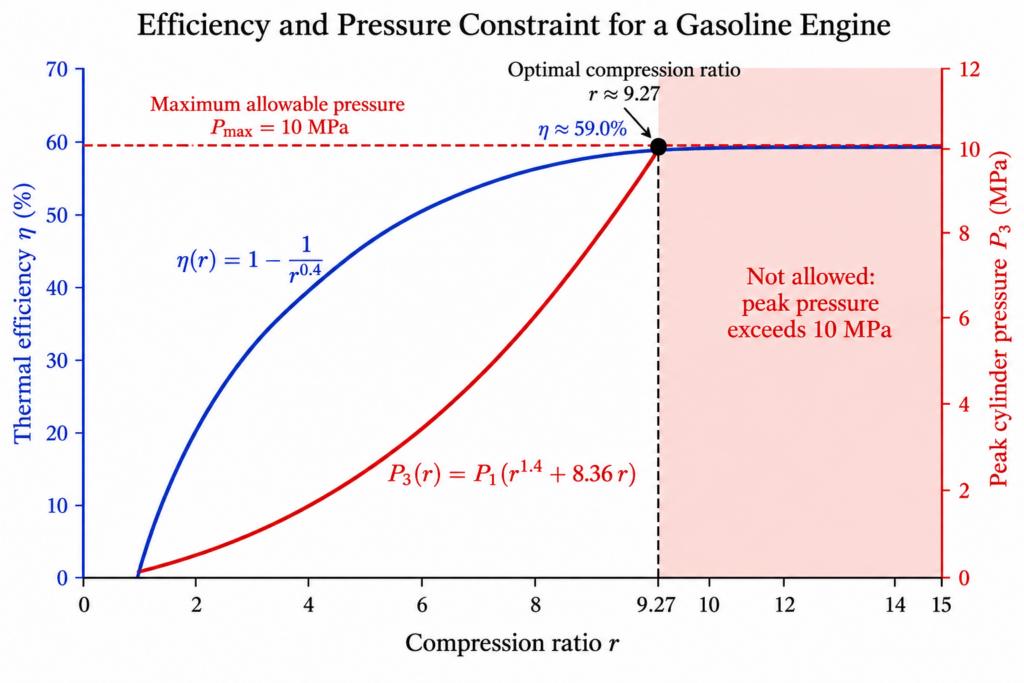
Using $γ = 1.4$ , the optimal compression ratio satisfies
$r^{1.4} + 8.36 r = 100 .$
Solving this equation numerically gives
$r \approx 9.27 .$
Thus, in this simplified model, the greatest possible efficiency under the pressure restriction occurs at a compression ratio of approximately 9.27:1.

What efficiency does this give?

For $γ = 1.4$ , the ideal Otto-cycle efficiency is
$η = 1 - \frac{1}{r^{0.4}} .$
Using $r \approx 9.27$ ,
$η \approx 1 - \frac{1}{{9.27}^{0.4}} \approx 0.590 .$
So the theoretical efficiency is approximately
$η \approx 59.0 % .$
This is the efficiency of the idealized mathematical model, not the efficiency we should expect from a real gasoline engine. Real engines have friction, heat loss, pumping losses, finite combustion time, changing specific heats, and other effects that the ideal Otto cycle does not include.

An unexpected seventh-degree polynomial

There is one more mathematical surprise.

We used
$γ = 1.4 = \frac{7}{5} .$
Therefore the equation determining the optimal compression ratio has the form
$r^{\frac{7}{5}} + B r = A .$
Let
$x = r^{\frac{1}{5}} .$
Then
$r = x^{5}$
and
$r^{\frac{7}{5}} = x^{7} .$
So our engine-design equation becomes
$x^{7} + B x^{5} - A = 0 .$
For our numerical example,
$x^{7} + 8.36 x^{5} - 100 = 0 .$
A practical question about the design of a gasoline engine has led us to a seventh-degree polynomial.

We do not need to solve this polynomial symbolically. A numerical method gives the physically relevant positive root and therefore the optimal compression ratio.

The mathematical lesson

Without a pressure restriction, the ideal Otto model says

larger compression ratio → greater efficiency.

There is no finite optimum.

But an engine has to withstand the pressure produced inside its cylinder. Once we impose the constraint
$P_{3} \leq P_{max},$
the optimization problem has a finite solution.

The optimum occurs precisely when increasing the compression ratio any further would violate the pressure constraint:
$P_{3} = P_{max} .$
This illustrates an important idea in applied calculus: sometimes the optimum is not created by a critical point of the function—it is created by the constraint.

Graph showing thermal efficiency and peak cylinder pressure versus compression ratio, with the optimal compression ratio of 9.27 determined by the 10 MPa pressure constraint.

September 27, 2026