The sliding-ladder problem is one of the most familiar examples of related rates in calculus.
A ladder leans against a vertical wall. The bottom begins to slide away from the wall, while the top slides downward.
Usually the textbook asks:
How fast is the top of the ladder moving?
But there is a more interesting question:
If you were on the ladder when it started to slide, what would the mathematics predict as the ladder approached the floor?
The answer is surprising.
The Geometry
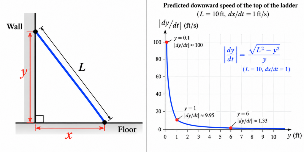
Suppose the ladder has fixed length L. Let x be the distance from the bottom of the ladder to the wall, and let y be the height of the top of the ladder above the floor.
Because the ladder, wall, and floor form a right triangle,
As the ladder slides, both x and y change with time. Differentiate with respect to t:
Dividing by 2 gives
Therefore,
This is the standard related-rates formula for a sliding ladder.
Suppose the Bottom Moves at Constant Speed
Assume that the bottom of the ladder moves away from the wall at a constant speed v:
Then
Since
we can also write
The minus sign tells us that the top of the ladder is moving downward.
What Happens Near the Floor?
As the top of the ladder approaches the floor,
Therefore,
and consequently
According to this model, the top of the ladder moves downward faster and faster, and its vertical speed becomes arbitrarily large as it approaches the floor.
A Numerical Example
Suppose the ladder is 10 feet long and its bottom slides away from the wall at
When the top is 6 feet above the floor,
Thus,
Nothing dramatic yet. But when the top is only 1 foot above the floor,
so
When the top is only 0.1 foot above the floor,
The closer the top gets to the floor, the larger the predicted downward speed becomes.
What About dy/dx?
There is another way to see where this strange behavior comes from. Differentiate
with respect to x. We obtain
and therefore
As the ladder approaches the floor,
Geometrically, this makes sense. The point moves along the quarter-circle
which has a vertical tangent at .
But there is an important distinction: dy/dx is not a velocity.
The connection with velocity is
If the horizontal speed remains positive and constant while becomes unbounded, then the predicted vertical velocity becomes unbounded as well.
So Is It Better to Slide or Jump?
At first sight, the mathematics seems to give a disturbing answer. If you remain with the ladder, the simple model predicts that the downward speed can become enormous near the floor.
Does that mean you should jump?
Not so fast.
The calculation has actually revealed something more interesting: the mathematical model has become physically unrealistic.
We assumed that the bottom of the ladder continues moving horizontally at a constant speed all the way until the ladder becomes horizontal. A real ladder cannot behave this way.
A real ladder has mass and rotational inertia. There is friction between the ladder and the floor and between the ladder and the wall. The ladder may lose contact with the wall. A person standing on it changes the center of mass and the forces acting on the system.
Most importantly, a real physical system cannot produce the infinite vertical velocity predicted by this simplified model.
So the infinity does not tell us that a real person will hit the floor at infinite speed.
It tells us that one of our assumptions must fail before that happens.
Calculus as a Warning About a Model
This is what makes the sliding-ladder problem more interesting than the usual textbook exercise.
Related rates correctly tells us that
Under the additional assumption that the horizontal speed stays constant, it follows that
The calculus is not wrong. The assumption is unrealistic.
When a correct calculation produces a physically impossible result, the mathematics may be telling us where our model stops being valid.
The humble sliding-ladder problem is therefore not just an exercise in implicit differentiation. It is also a lesson about the difference between mathematics and the physical world.
Related: Another example of mathematics revealing the limitations of a model is Population Growth: From Exponential Growth to the Logistic Equation .
For another example of how calculus models motion in the real world, see Projectile Motion in 3D: Adding Wind and Air Resistance, where the standard projectile problem is extended to include wind and air resistance.
Another classical motion problem with a surprising answer is the brachistochrone problem. The fastest path is a cycloid when there is no resistance—but what happens when fluid resistance is added?
Calculus describes many kinds of motion, from mechanical systems on Earth to planets orbiting the Sun. For a fascinating application of derivatives, geometry, and Newton’s laws, read Kepler’s Laws: How Calculus Explains Planetary Motion .