Tag: Parametric Equations

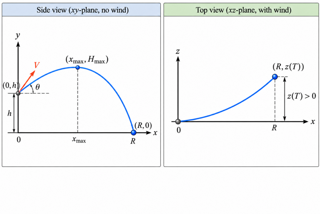
The standard projectile-motion problem is familiar from calculus and physics: a projectile is launched with initial speed V at an angle θ above the horizontal from an initial height h. Gravity pulls it downward, and we ask two basic questions:

• How high does the projectile go?
• How far does it travel before hitting the ground?

But real projectiles do not necessarily stay in a vertical plane. What happens if we add a horizontal wind blowing from the side? And what happens if we also include air resistance?

The familiar two-dimensional parabola becomes a genuinely three-dimensional trajectory. With a simple model of air resistance, we can still obtain explicit formulas for almost everything.

1. Setting Up the Coordinates

Choose coordinates so that:

• x is the original horizontal firing direction,
• y is the vertical direction,
• z is the sideways horizontal direction.

The projectile is fired in the vertical xy-plane, so initially there is no velocity in the z-direction.

The initial position is

$$\mathbf{r}\left(0\right)=(0,h,0).$$

The initial velocity is

$$\mathbf{v}\left(0\right)=(V\cos \theta ,V\sin \theta ,0).$$

2. Adding Wind

Suppose a horizontal wind has speed W and makes an angle φ with the positive x-direction. Its velocity vector is

$$\mathbf{w}=(W\cos \phi ,0,W\sin \phi ).$$

The component $W\cos \phi$ pushes along the original firing direction, while $W\sin \phi$ produces sideways motion.

3. Air Resistance Must Be Relative to the Air

If there were no air resistance, a steady wind would have no effect on an ideal point projectile. Wind matters because the projectile interacts with the surrounding air.

For a simple model, assume that air resistance is proportional to the projectile’s velocity relative to the moving air. If k is the drag constant per unit mass, the acceleration due to air resistance is

$$-k(\mathbf{v}-\mathbf{w}).$$

Gravity contributes

$$(0,-g,0).$$

Therefore the equation of motion is

$${\mathbf{r}}^{″}=-g\mathbf{j}-k({\mathbf{r}}^{\prime }-\mathbf{w}).$$

4. Three Differential Equations

Writing the vector equation component by component gives

$$\begin{array}{rcl}{x}^{″}& =& -k(x^{\prime }-W\cos \phi )\\ y^{″}& =& -g-k{y}^{\prime }\\ z^{″}& =& -k(z^{\prime }-W\sin \phi ).\end{array}$$

Although the trajectory is three-dimensional, something very convenient has happened: the three equations can be solved separately.

5. Solving for the Velocity

The velocity in the x-direction is

$$v_x\left(t\right)=W\cos \phi +(V\cos \theta -W\cos \phi )e^{-kt}.$$

The sideways velocity is

$$v_z\left(t\right)=W\sin \phi (1-e^{-kt}).$$

The vertical velocity is

$$v_y\left(t\right)=(V\sin \theta +\frac{g}{k})e^{-kt}-\frac{g}{k}.$$

Notice the long-term behavior. The horizontal velocity approaches the wind velocity, while the vertical velocity approaches

$$-\frac{g}{k}.$$

In this linear-drag model, this is the terminal vertical velocity.

6. The 3D Position

Integrating the velocity components and using the initial position gives

$$x\left(t\right)=W\cos \phi t+\frac{V\cos \theta -W\cos \phi }{k}(1-e^{-kt}).$$ $$y\left(t\right)=h-\frac{g}{k}t+\frac{V\sin \theta +\frac{g}{k}}{k}(1-e^{-kt}).$$ $$z\left(t\right)=W\sin \phi [t-\frac{1-e^{-kt}}{k}].$$

These three equations describe the complete trajectory through space. Unlike the usual projectile trajectory, this curve is not a parabola.

7. When Does the Projectile Reach Its Maximum Height?

At maximum height the vertical velocity is zero:

$$v_y\left(t_{\max }\right)=0.$$

Therefore

$$(V\sin \theta +\frac{g}{k})e^{-k{t}_{\max }}=\frac{g}{k}.$$

Solving for time gives

$$t_{\max }=\frac{1}{k}\ln (1+\frac{kV\sin \theta }{g}).$$

8. Maximum Height

Substituting this time into the vertical position formula and simplifying gives

$$H_{\max }=h+\frac{V\sin \theta }{k}-\frac{g}{k^2}\ln (1+\frac{kV\sin \theta }{g}).$$

An interesting consequence is that the horizontal wind does not appear in this formula. In this model, horizontal wind changes where the projectile lands, but it does not change its maximum height.

9. When Does It Hit the Ground?

Let T denote the time at which the projectile hits the ground. We find T by setting

$$y\left(T\right)=0.$$

Thus T satisfies

$$h-\frac{g}{k}T+\frac{V\sin \theta +\frac{g}{k}}{k}(1-e^{-kT})=0.$$

Here we encounter an important difference from the standard projectile problem. Without air resistance, finding the flight time requires solving a quadratic equation. With linear air resistance, the unknown T appears both outside and inside an exponential.

In practice, the positive solution can be found numerically using a calculator, computer, graphing program, or Newton’s method.

10. Where Does It Land?

Once the flight time T has been found, the landing point is

$$\left(x\right(T),0,z(T\left)\right).$$

The downrange distance in the original firing direction is $x\left(T\right)$, while the sideways displacement is $z\left(T\right)$.

The total horizontal distance between the launch point and landing point is

$$R=\sqrt{{x\left(T\right)}^2+{z\left(T\right)}^2}.$$

So in three dimensions, the question “How far does the projectile go?” has more than one possible answer. We can ask for its downrange distance, its sideways drift, or its total horizontal displacement.

11. How Far Sideways Does the Wind Push It?

The sideways displacement at landing is

$$z\left(T\right)=W\sin \phi [T-\frac{1-e^{-kT}}{k}].$$

This is zero when the wind blows exactly along the original firing direction. It becomes nonzero when the wind has a crosswind component.

12. A Consistency Check: Remove Air Resistance

A good mathematical model should reproduce the familiar result when the new effect is removed. Let the drag coefficient k approach zero. A key limit is

$$\underset{k\to 0}{\lim }\frac{1-e^{-kt}}{k}=t.$$

As air resistance disappears, the vertical motion approaches

$$y\left(t\right)=h+V\sin \theta t-\frac{1}{2}g{t}^2,$$

which is exactly the standard projectile-motion formula.

The maximum-height formula also approaches

$$H_{\max }\to h+\frac{V^2{\sin \theta }^2}{2g}.$$

Again, this is precisely the familiar result.

13. From a Parabola to a Space Curve

The ordinary projectile problem is two-dimensional. Its trajectory is a parabola contained in a vertical plane.

Adding a crosswind and air resistance changes the geometry completely. The projectile now moves simultaneously forward, vertically, and sideways. Its position is described parametrically by

$$\mathbf{r}\left(t\right)=\left(x\right(t),y(t),z(t\left)\right).$$

This is a natural example of why parametric vector equations are useful: there is no need to force a three-dimensional trajectory into a single equation involving x, y, and z.

14. What Makes This Problem Interesting?

The standard projectile problem is often presented as an application of quadratic functions. But a relatively small change in the physical assumptions leads to much richer mathematics.

The three-dimensional model combines:

• vectors and parametric curves,
• differential equations,
• exponential functions,
• optimization,
• numerical root finding,
• limits,
• and mathematical modeling.

Most importantly, the model separates two questions that look similar but are physically different. Gravity and vertical drag determine when the projectile hits the ground. The wind and horizontal drag then determine where it lands.

That is the real advantage of moving from the familiar two-dimensional projectile problem to a three-dimensional model: instead of asking only “How far?”, we can ask the more interesting question: Where will it land?

Worked Example: Where Does the Projectile Land?

Let us use the formulas above with actual numbers. Suppose a projectile is launched from a height of 10 meters with an initial speed of 40 m/s at an angle of 45° above the horizontal.

A horizontal wind blows at 10 m/s at an angle of 60° from the original firing direction. Assume a linear drag constant k = 0.10 s⁻¹ and take g = 9.81 m/s².

Thus our data are

$$h=10\text{m},\hspace{1em}V=40\text{m/s},\hspace{1em}\theta ={45}^{°},$$ $$W=10\text{m/s},\hspace{1em}\phi ={60}^{°},\hspace{1em}k=0.10\text{s}{}^{-1}.$$

Step 1: When Does It Reach Maximum Height?

The time at which the projectile reaches its maximum height is

$$t_{\max }=\frac{1}{k}\ln (1+\frac{kV\sin \theta }{g}).$$

Substituting the numerical values gives

$$t_{\max }=\frac{1}{0.10}\ln (1+\frac{\left(0.10\right)\left(40\right)\sin {45}^{°}}{9.81}).$$

Therefore,

$$t_{\max }\approx 2.533\text{s}.$$

The projectile reaches its highest point about 2.53 seconds after launch.

Step 2: What Is the Maximum Height?

The maximum height is

$$H_{\max }=h+\frac{V\sin \theta }{k}-\frac{g}{k^2}\ln (1+\frac{kV\sin \theta }{g}).$$

Substitution gives

$$H_{\max }=10+\frac{40\sin {45}^{°}}{0.10}-\frac{9.81}{{0.10}^2}\ln (1+\frac{\left(0.10\right)\left(40\right)\sin {45}^{°}}{9.81}).$$

Thus

$$H_{\max }\approx 44.32\text{m}.$$

The projectile rises to approximately 44.32 meters above the ground.

Step 3: When Does It Hit the Ground?

The projectile hits the ground when $y\left(T\right)=0$. For our values, this means solving

$$10-\frac{9.81}{0.10}T+\frac{40\sin {45}^{°}+\frac{9.81}{0.10}}{0.10}(1-e^{-0.10T})=0.$$

Unlike the standard projectile problem, this is not a quadratic equation. The unknown T appears both by itself and in an exponential. Solving the equation numerically gives

$$T\approx 5.698\text{s}.$$

So the projectile is in the air for approximately 5.70 seconds.

Step 4: How Far Downrange Does It Travel?

The horizontal x-coordinate at landing is

$$x\left(T\right)=W\cos \phi T+\frac{V\cos \theta -W\cos \phi }{k}(1-e^{-kT}).$$

Substituting $T\approx 5.698$ gives

$$x\left(T\right)\approx 129.62\text{m}.$$

Thus the projectile travels approximately 129.62 meters downrange.

Step 5: How Far Sideways Does the Wind Push It?

The sideways coordinate at landing is

$$z\left(T\right)=W\sin \phi [T-\frac{1-e^{-kT}}{k}].$$

Substituting the numerical values gives

$$z\left(T\right)=10\sin {60}^{°}[5.698-\frac{1-e^{-\left(0.10\right)\left(5.698\right)}}{0.10}].$$

Therefore,

$$z\left(T\right)\approx 11.73\text{m}.$$

The wind has pushed the projectile approximately 11.73 meters sideways from the original vertical firing plane.

Step 6: Where Does It Land?

We now know both horizontal coordinates. Therefore the landing point is approximately

$$\mathbf{P}=(129.62,0,11.73)\text{m}.$$

In other words, the projectile lands approximately 129.62 meters downrange and 11.73 meters sideways from the original vertical firing plane.

Step 7: Total Horizontal Displacement

The straight-line horizontal distance from the point directly below the launch position to the landing point is

$$R=\sqrt{{x\left(T\right)}^2+{z\left(T\right)}^2}.$$

Therefore,

$$R=\sqrt{{129.62}^2+{11.73}^2}\approx 130.15\text{m}.$$

The Answer

For this example, the projectile reaches a maximum height of approximately 44.32 m and stays in the air for approximately 5.70 s.

It lands approximately 129.62 m downrange and 11.73 m sideways from the original vertical firing plane. Thus its landing point is

$$(129.62,0,11.73)\text{m}.$$

The total horizontal displacement from the point directly below the launch position is approximately 130.15 m. The sideways displacement shows exactly how the wind changes the familiar two-dimensional projectile problem into a three-dimensional one.

---

For another example of how calculus can reveal something unexpected in a real-world motion problem, see Sliding Ladder: Is It Better to Slide or Jump?.

Projectile motion and planetary motion are both governed by Newton’s laws. Near Earth’s surface, gravity is approximately constant, while planetary orbits require the inverse-square law of gravitation. Explore this connection in Kepler’s Laws: How Calculus Explains Planetary Motion .