Elite Math Program

Tag: Multivariable calculus

Projectile Motion in 3D: Adding Wind and Air Resistance
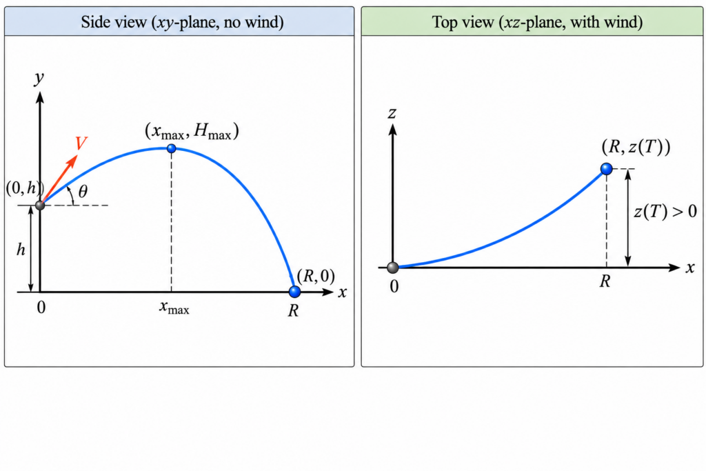
The standard projectile-motion problem is familiar from calculus and physics: a projectile is launched with initial speed V at an angle θ above the horizontal from an initial height h. Gravity pulls it downward, and we ask two basic questions:
- How high does the projectile go?
- How far does it travel before hitting the ground?
But real projectiles do not necessarily stay in a vertical plane. What happens if we add a horizontal wind blowing from the side? And what happens if we also include air resistance?

The familiar two-dimensional parabola becomes a genuinely three-dimensional trajectory. With a simple model of air resistance, we can still obtain explicit formulas for almost everything.

1. Setting Up the Coordinates

Choose coordinates so that:
- x is the original horizontal firing direction,
- y is the vertical direction,
- z is the sideways horizontal direction.
The projectile is fired in the vertical xy-plane, so initially there is no velocity in the z-direction.

The initial position is
r (0) = ( 0,h,0 ).
The initial velocity is
v (0) = ( V⁢cos⁡θ , V⁢sin⁡θ ,0 ).
2. Adding Wind

Suppose a horizontal wind has speed W and makes an angle φ with the positive x-direction. Its velocity vector is
w= ( W⁢cos⁡φ ,0, W⁢sin⁡φ ).
The component $W \cos φ$ pushes along the original firing direction, while $W \sin φ$ produces sideways motion.

3. Air Resistance Must Be Relative to the Air

If there were no air resistance, a steady wind would have no effect on an ideal point projectile. Wind matters because the projectile interacts with the surrounding air.

For a simple model, assume that air resistance is proportional to the projectile’s velocity relative to the moving air. If k is the drag constant per unit mass, the acceleration due to air resistance is
−k ( v − w ).
Gravity contributes
( 0,−g,0 ).
Therefore the equation of motion is
r″ = −gj −k ( r′ − w ).
4. Three Differential Equations

Writing the vector equation component by component gives
x″ = −k ( x′ − W⁢cos⁡φ ) y″ = −g −ky′ z″ = −k ( z′ − W⁢sin⁡φ ).
Although the trajectory is three-dimensional, something very convenient has happened: the three equations can be solved separately.

5. Solving for the Velocity

The velocity in the x-direction is
vx (t) = W⁢cos⁡φ + ( V⁢cos⁡θ − W⁢cos⁡φ ) e−kt.
The sideways velocity is
vz (t) = W⁢sin⁡φ ( 1− e−kt ).
The vertical velocity is
vy (t) = ( V⁢sin⁡θ + gk ) e−kt − gk.
Notice the long-term behavior. The horizontal velocity approaches the wind velocity, while the vertical velocity approaches
−gk.
In this linear-drag model, this is the terminal vertical velocity.

6. The 3D Position

Integrating the velocity components and using the initial position gives
x (t) = W⁢cos⁡φt + V⁢cos⁡θ − W⁢cos⁡φ k ( 1− e−kt ). y (t) = h − gkt + V⁢sin⁡θ +gk k ( 1− e−kt ). z (t) = W⁢sin⁡φ [ t − 1− e−kt k ].
These three equations describe the complete trajectory through space. Unlike the usual projectile trajectory, this curve is not a parabola.

7. When Does the Projectile Reach Its Maximum Height?

At maximum height the vertical velocity is zero:
vy ( tmax ) =0.
Therefore
( V⁢sin⁡θ +gk ) e −ktmax = gk.
Solving for time gives
tmax = 1k ln⁡ ( 1 + kV⁢sin⁡θ g ).
8. Maximum Height

Substituting this time into the vertical position formula and simplifying gives
Hmax = h + V⁢sin⁡θ k − gk2 ln⁡ ( 1 + kV⁢sin⁡θ g ).
An interesting consequence is that the horizontal wind does not appear in this formula. In this model, horizontal wind changes where the projectile lands, but it does not change its maximum height.

9. When Does It Hit the Ground?

Let T denote the time at which the projectile hits the ground. We find T by setting
y (T) =0.
Thus T satisfies
h − gkT + V⁢sin⁡θ + gk k ( 1− e−kT ) =0.
Here we encounter an important difference from the standard projectile problem. Without air resistance, finding the flight time requires solving a quadratic equation. With linear air resistance, the unknown T appears both outside and inside an exponential.

In practice, the positive solution can be found numerically using a calculator, computer, graphing program, or Newton’s method.

10. Where Does It Land?

Once the flight time T has been found, the landing point is
( x(T) , 0 , z(T) ).
The downrange distance in the original firing direction is $x (T)$ , while the sideways displacement is $z (T)$ .

The total horizontal distance between the launch point and landing point is
R= x(T) 2 + z(T) 2 .
So in three dimensions, the question “How far does the projectile go?” has more than one possible answer. We can ask for its downrange distance, its sideways drift, or its total horizontal displacement.

11. How Far Sideways Does the Wind Push It?

The sideways displacement at landing is
z (T) = W⁢sin⁡φ [ T − 1− e−kT k ].
This is zero when the wind blows exactly along the original firing direction. It becomes nonzero when the wind has a crosswind component.

12. A Consistency Check: Remove Air Resistance

A good mathematical model should reproduce the familiar result when the new effect is removed. Let the drag coefficient k approach zero. A key limit is
lim k→0 1− e−kt k =t.
As air resistance disappears, the vertical motion approaches
y (t) = h + V⁢sin⁡θt − 12 gt2,
which is exactly the standard projectile-motion formula.

The maximum-height formula also approaches
Hmax → h + V2 sin⁡θ 2 2g .
Again, this is precisely the familiar result.

13. From a Parabola to a Space Curve

The ordinary projectile problem is two-dimensional. Its trajectory is a parabola contained in a vertical plane.

Adding a crosswind and air resistance changes the geometry completely. The projectile now moves simultaneously forward, vertically, and sideways. Its position is described parametrically by
r (t) = ( x(t) , y(t) , z(t) ).
This is a natural example of why parametric vector equations are useful: there is no need to force a three-dimensional trajectory into a single equation involving x, y, and z.

14. What Makes This Problem Interesting?

The standard projectile problem is often presented as an application of quadratic functions. But a relatively small change in the physical assumptions leads to much richer mathematics.

The three-dimensional model combines:
- vectors and parametric curves,
- differential equations,
- exponential functions,
- optimization,
- numerical root finding,
- limits,
- and mathematical modeling.
Most importantly, the model separates two questions that look similar but are physically different. Gravity and vertical drag determine when the projectile hits the ground. The wind and horizontal drag then determine where it lands.

That is the real advantage of moving from the familiar two-dimensional projectile problem to a three-dimensional model: instead of asking only “How far?”, we can ask the more interesting question: Where will it land?

Worked Example: Where Does the Projectile Land?

Let us use the formulas above with actual numbers. Suppose a projectile is launched from a height of 10 meters with an initial speed of 40 m/s at an angle of 45° above the horizontal.

A horizontal wind blows at 10 m/s at an angle of 60° from the original firing direction. Assume a linear drag constant k = 0.10 s⁻¹ and take g = 9.81 m/s².

Thus our data are
h=10 m, V=40 m/s, θ=45°, W=10 m/s, φ=60°, k=0.10 s −1.
Step 1: When Does It Reach Maximum Height?

The time at which the projectile reaches its maximum height is
tmax = 1k ln⁡ ( 1 + kV ⁢ sin⁡θ g ).
Substituting the numerical values gives
tmax = 10.10 ln⁡ ( 1 + ( 0.10 ) ( 40 ) sin⁡ 45° 9.81 ).
Therefore,
tmax ≈ 2.533 s.
The projectile reaches its highest point about 2.53 seconds after launch.

Step 2: What Is the Maximum Height?

The maximum height is
Hmax = h + V ⁢ sin⁡θ k − g k2 ln⁡ ( 1 + kV ⁢ sin⁡θ g ).
Substitution gives
Hmax = 10 + 40 sin⁡ 45° 0.10 − 9.81 0.102 ln⁡ ( 1 + ( 0.10 ) ( 40 ) sin⁡ 45° 9.81 ).
Thus
Hmax ≈ 44.32 m.
The projectile rises to approximately 44.32 meters above the ground.

Step 3: When Does It Hit the Ground?

The projectile hits the ground when $y (T) = 0$ . For our values, this means solving
10 − 9.810.10T + 40 sin⁡ 45° + 9.810.10 0.10 ( 1 − e −0.10T ) =0.
Unlike the standard projectile problem, this is not a quadratic equation. The unknown T appears both by itself and in an exponential. Solving the equation numerically gives
T ≈ 5.698 s.
So the projectile is in the air for approximately 5.70 seconds.

Step 4: How Far Downrange Does It Travel?

The horizontal x-coordinate at landing is
x ( T ) = W ⁢ cos⁡φ ⁢T + V ⁢ cos⁡θ − W ⁢ cos⁡φ k ( 1 − e −kT ).
Substituting $T \approx 5.698$ gives
x ( T ) ≈ 129.62 m.
Thus the projectile travels approximately 129.62 meters downrange.

Step 5: How Far Sideways Does the Wind Push It?

The sideways coordinate at landing is
z ( T ) = W ⁢ sin⁡φ [ T − 1 − e −kT k ].
Substituting the numerical values gives
z ( T ) = 10 sin⁡ 60° [ 5.698 − 1 − e − ( 0.10 ) ( 5.698 ) 0.10 ].
Therefore,
z ( T ) ≈ 11.73 m.
The wind has pushed the projectile approximately 11.73 meters sideways from the original vertical firing plane.

Step 6: Where Does It Land?

We now know both horizontal coordinates. Therefore the landing point is approximately
P = ( 129.62 , 0 , 11.73 ) m.
In other words, the projectile lands approximately 129.62 meters downrange and 11.73 meters sideways from the original vertical firing plane.

Step 7: Total Horizontal Displacement

The straight-line horizontal distance from the point directly below the launch position to the landing point is
R = x ( T ) 2 + z ( T ) 2 .
Therefore,
R = 129.622 + 11.732 ≈ 130.15 m.
The Answer

For this example, the projectile reaches a maximum height of approximately 44.32 m and stays in the air for approximately 5.70 s.

It lands approximately 129.62 m downrange and 11.73 m sideways from the original vertical firing plane. Thus its landing point is
( 129.62 , 0 , 11.73 ) m.
The total horizontal displacement from the point directly below the launch position is approximately 130.15 m. The sideways displacement shows exactly how the wind changes the familiar two-dimensional projectile problem into a three-dimensional one.

For another example of how calculus can reveal something unexpected in a real-world motion problem, see Sliding Ladder: Is It Better to Slide or Jump?.

Projectile motion and planetary motion are both governed by Newton’s laws. Near Earth’s surface, gravity is approximately constant, while planetary orbits require the inverse-square law of gravitation. Explore this connection in Kepler’s Laws: How Calculus Explains Planetary Motion .
October 3, 2026
Proving 1 + 1/4 + 1/9 + ⋯ = π²/6 with a Double Integral

One of the most famous identities in mathematics is
$1 + \frac{1}{4} + \frac{1}{9} + \frac{1}{16} + \dots = \frac{π^{2}}{6} .$
In summation notation,
$\sum_{n = 1}^{\infty} \frac{1}{n^{2}} = \frac{π^{2}}{6} .$
This is known as the Basel problem. Euler famously solved it in the eighteenth century. There are many proofs, but one particularly beautiful approach uses a double integral and an unexpected change of variables.

Start with the odd terms

Instead of attacking the entire series immediately, consider only the reciprocals of the odd squares:
$S = 1 + \frac{1}{3^{2}} + \frac{1}{5^{2}} + \frac{1}{7^{2}} + \dots .$
We will first prove that
$S = \frac{π^{2}}{8} .$
The full Basel sum will then follow almost immediately.

Turn the series into a double integral

Consider
$I = \int_{0}^{1} \int_{0}^{1} \frac{1}{1 - x^{2} y^{2}} d x d y .$
For points inside the unit square, the geometric-series identity gives
$\frac{1}{1 - x^{2} y^{2}} = \sum_{n = 0}^{\infty} {x y}^{2 n} .$
Therefore,
$I = \sum_{n = 0}^{\infty} (\int_{0}^{1} x^{2 n} d x) (\int_{0}^{1} y^{2 n} d y) .$
Each one-dimensional integral is
$\int_{0}^{1} x^{2 n} d x = \frac{1}{2 n + 1} .$
Hence
$I = \sum_{n = 0}^{\infty} \frac{1}{{(2 n + 1)}^{2}} .$
Thus the double integral is exactly the sum of the reciprocals of the odd squares:
$I = 1 + \frac{1}{3^{2}} + \frac{1}{5^{2}} + \dots .$
The key change of variables

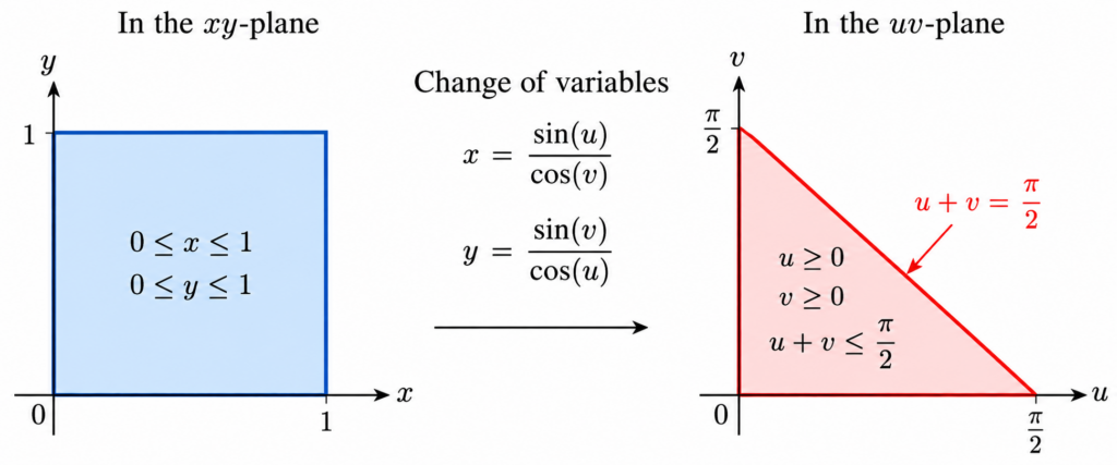
Now comes the surprising part. Introduce new variables u and v by
$x = \frac{\sin (u)}{\cos (v)}, y = \frac{\sin (v)}{\cos (u)} .$
The square
$0 \leq x \leq 1, 0 \leq y \leq 1$
corresponds to the triangular region
$u \geq 0, v \geq 0, u + v \leq \frac{π}{2} .$
To see where the last boundary comes from, notice that
$x \leq 1 \Leftrightarrow \sin (u) \leq \cos (v) \Leftrightarrow u + v \leq \frac{π}{2},$
and the condition on y gives the same inequality.

The Jacobian

We compute
$\frac{\partial x}{\partial u} = \frac{\cos (u)}{\cos (v)}, \frac{\partial x}{\partial v} = \frac{\sin (u) \sin (v)}{{\cos (v)}^{2}} .$
Similarly,
$\frac{\partial y}{\partial u} = \frac{\sin (u) \sin (v)}{{\cos (u)}^{2}}, \frac{\partial y}{\partial v} = \frac{\cos (v)}{\cos (u)} .$
After simplifying the determinant, the Jacobian is
$\frac{\partial (x, y)}{\partial (u, v)} = 1 - x^{2} y^{2} .$
This is exactly the expression that appears in the denominator of our original integral. Therefore,
$\frac{d x d y}{1 - x^{2} y^{2}} = d u d v .$
The complicated-looking integrand has completely disappeared.

The integral becomes an area

Our double integral is now simply
$I = \int_{0}^{\frac{π}{2}} \int_{0}^{\frac{π}{2} - u} d v d u .$
Geometrically, this is the area of a right triangle whose two perpendicular sides both have length
$\frac{π}{2}$
Therefore,
$I = \frac{1}{2} \cdot \frac{π}{2} \cdot \frac{π}{2} = \frac{π^{2}}{8} .$
We have proved that
$1 + \frac{1}{3^{2}} + \frac{1}{5^{2}} + \frac{1}{7^{2}} + \dots = \frac{π^{2}}{8} .$
Recovering the full series

Let
$T = \sum_{n = 1}^{\infty} \frac{1}{n^{2}} .$
Split the series into its odd and even terms. The odd terms have sum
$\frac{π^{2}}{8}$
while the even terms have sum
$\frac{1}{2^{2}} + \frac{1}{4^{2}} + \frac{1}{6^{2}} + \dots = \frac{1}{4} T .$
Consequently,
$T = \frac{π^{2}}{8} + \frac{1}{4} T .$
Thus,
$\frac{3}{4} T = \frac{π^{2}}{8},$
and finally,
$T = \frac{π^{2}}{6} .$
Why this proof is remarkable

We started with an infinite series involving nothing but reciprocals of squares. We then represented part of that series by a double integral over a square. A carefully chosen trigonometric change of variables transformed the square into a triangle and, at the same time, made the integrand disappear.

The infinite series was therefore reduced to the area of a triangle:
$\frac{1}{2} \cdot \frac{π}{2} \cdot \frac{π}{2} = \frac{π^{2}}{8} .$
From there, separating the odd and even terms gives the celebrated result
$\sum_{n = 1} \frac{1}{n^{2}} = \frac{π^{2}}{6} .$
It is a striking example of how an infinite series, a double integral, a trigonometric substitution, and a simple geometric area can all describe the same number.

Another Problem Where Two Dimensions Help

The double-integral proof of the Basel sum illustrates a powerful mathematical idea: sometimes a problem becomes easier when we move to a higher dimension.

One of the most beautiful examples is the Gaussian integral. A one-dimensional integral that resists ordinary antiderivative methods becomes accessible after it is squared and transformed into a two-dimensional integral.

Continue exploring: The Gaussian Integral and Beyond: From e^(-x²) to a Family of Integrals

Long before Euler solved the Basel problem, ancient Greek mathematicians had developed ingenious geometric methods for evaluating infinite sums. In particular, Archimedes used areas of triangles to establish a remarkable infinite series identity. Discover his method in How the Ancient Greeks Summed Infinite Series Without Calculus .

September 28, 2026
Why the Equilateral Triangle Wins: Maximum Area for a Fixed Perimeter

Suppose you have a fixed length of wire and want to bend it into a triangle. Which triangle encloses the largest possible area?

It is natural to guess that the answer is the equilateral triangle. But why? This is a beautiful example of how a geometric optimization problem can be turned into a multivariable calculus problem and solved using Lagrange multipliers.

Setting up the problem

Let the side lengths of the triangle be
$a, b, c .$
Suppose the perimeter is fixed and equal to $P$ . Thus,
$a + b + c = P .$
We want to determine which values of $a$ , $b$ , and $c$ produce the largest possible area.

Heron’s formula

Let
$s = \frac{P}{2}$
be the semiperimeter. Heron’s formula can be written in squared form as
$A^{2} = s (s - a) (s - b) (s - c) .$
Because the perimeter is fixed, $s$ is also fixed. Moreover, maximizing $A$ is equivalent to maximizing $A^{2}$ . So this form of Heron’s formula is particularly convenient for our problem.

A useful change of variables

Introduce three new variables:
$x = s - a, y = s - b, z = s - c .$
The triangle inequalities imply that $x$ , $y$ , and $z$ are positive.

Adding the three equations gives
$x + y + z = 3 s - (a + b + c) .$
Since
$a + b + c = 2 s,$
we obtain the simple constraint
$x + y + z = s .$
Heron’s formula now becomes
$A^{2} = s x y z .$
Since $s$ is fixed, maximizing the area is equivalent to maximizing
$f (x, y, z) = x y z$
subject to
$x + y + z = s .$
The original geometry problem has therefore become a simple question: among three positive numbers with a fixed sum, when is their product largest?

Using Lagrange multipliers

Define
$f (x, y, z) = x y z$
and let the constraint function be
$g (x, y, z) = x + y + z .$
At a constrained maximum, the gradients of $f$ and $g$ must be parallel:
$\nabla f = λ \nabla g .$
We have
$\nabla f = ⟨ y z, x z, x y ⟩$
and
$\nabla g = ⟨ 1, 1, 1 ⟩ .$
Therefore, the Lagrange multiplier equations are
$y z = λ, x z = λ, x y = λ .$
Thus,
$y z = x z = x y .$
Since $x$ , $y$ , and $z$ are positive, these equations imply
$x = y = z .$
Their sum is $s$ , so
$x = y = z = \frac{s}{3} .$
Returning to the triangle

Recall that
$x = s - a, y = s - b, z = s - c .$
Since $x = y = z$ , we obtain
$a = b = c .$
Because the perimeter is $P$ , each side must therefore have length
$a = b = c = \frac{P}{3} .$
Therefore, the triangle of maximum area is the equilateral triangle.

What is the maximum area?

For an equilateral triangle with side length $\frac{P}{3}$ , the area is
$A_{max} = \frac{\sqrt{3}}{4} {(\frac{P}{3})}^{2} .$
Therefore,
$A_{max} = \frac{\sqrt{3} P^{2}}{36} .$
Why this argument is interesting

We started with a geometric question about triangles. Heron’s formula converted the area problem into an algebraic one. A simple change of variables then transformed it into the problem of maximizing the product of three positive numbers whose sum is fixed.

Lagrange multipliers reveal the symmetry automatically: at the maximum, the three variables must be equal. Translating that condition back into geometry tells us that the three sides of the triangle must also be equal.

This is one of the appealing features of multivariable calculus: a geometric statement that seems intuitively obvious emerges naturally from an optimization calculation.

Conclusion: Among all triangles with a fixed perimeter, the equilateral triangle has the largest area.

For another surprising connection between equilateral-triangle geometry and a classical geometric object, see The Steiner Inellipse and a Surprising Area Characterization .

The equilateral triangle is distinguished by its symmetry. In three dimensions, the regular tetrahedron has similar geometric elegance. Explore its face areas, volume, and a three-dimensional Pythagorean theorem in The Geometry of a Tetrahedron .

September 28, 2026
A Surprising Integral on the Sphere: Why Every Direction Is the Same
Consider the integral
I ( u ) = ∫ S n − 1 | u · x | d S ( x )
where $S^{n - 1}$ is the unit sphere in $R^{n}$ and $u$ is a fixed vector. At first glance, this looks like a difficult high-dimensional integral. The absolute value creates a nonsmooth integrand, but the symmetry of the sphere makes the calculation surprisingly simple.

The key observation

Write
u = ∥ u ∥ e
where $e$ is a unit vector. Then
| u · x | = ∥ u ∥ | e · x |
Therefore,
I ( u ) = ∥ u ∥ ∫ S n − 1 | e · x | d S ( x )
The remaining integral does not depend on the direction of $e$ . The sphere is rotationally symmetric, so we may rotate the coordinate system and assume that
e = ( 1 , 0 , … , 0 )
Then
e · x = x 1
and therefore
I ( u ) = ∥ u ∥ ∫ S n − 1 | x 1 | d S ( x )
A geometric interpretation

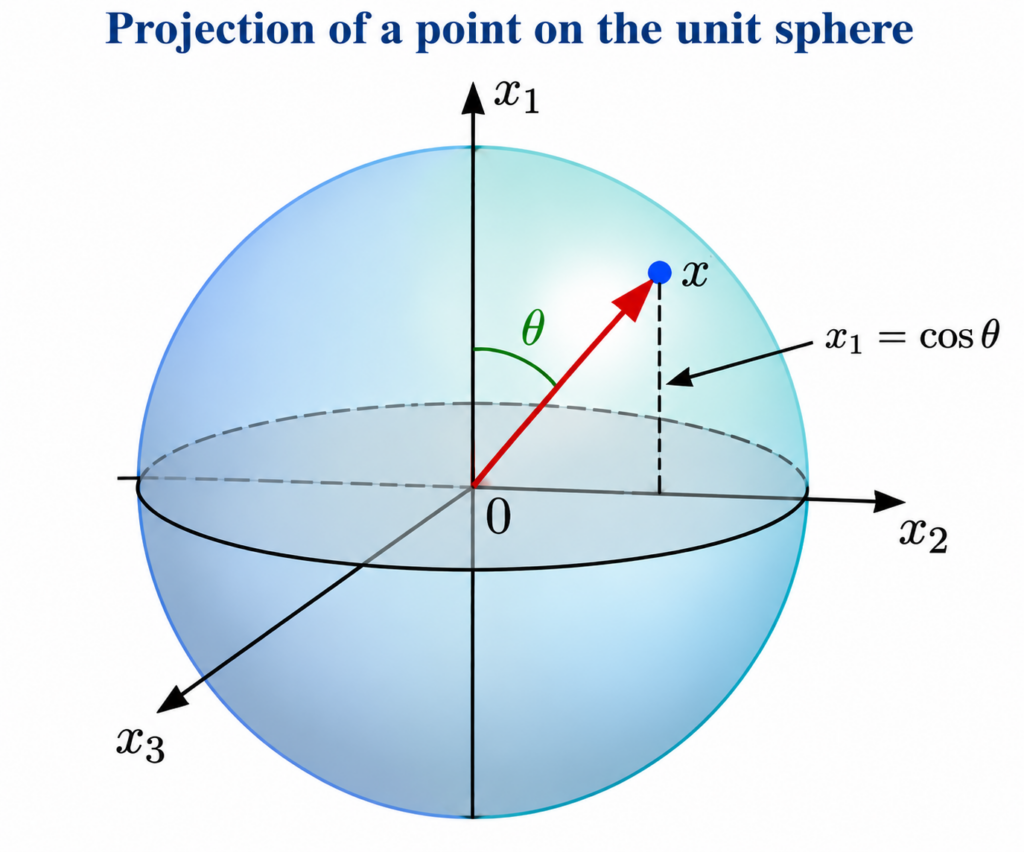
For a point $x$ on the sphere, let $θ$ be the angle between $x$ and the chosen direction $e$ . Then the projection of $x$ onto this direction is
e · x = cos ( θ )
so
| u · x | = ∥ u ∥ | cos ( θ ) |
The integral is therefore the total absolute projection of all points on the sphere onto a fixed direction.

Measuring spheres

The notation $| S^{n} |$ means the surface area of the unit sphere $S^{n}$ .

For example,
- $S^{0}$ consists of two points, so $| S^{0} | = 2$ .
- $S^{1}$ is the unit circle, so $| S^{1} | = 2 π$ .
- $S^{2}$ is the ordinary unit sphere, so $| S^{2} | = 4 π$ .
Now consider the sphere $S^{n - 1}$ . Fix the angle $θ$ between a point $x$ on this sphere and a fixed direction $e$ .

All points with the same angle $θ$ form a lower-dimensional sphere $S^{n - 2}$ . Therefore, $| S^{n - 2} |$ is the surface area of this slice of the sphere.

This is the geometric reason that $| S^{n - 2} |$ appears when we compute the integral using spherical coordinates.

The lower-dimensional sphere

To compute the integral, we slice the sphere by fixing the angle $θ$ . Each slice is itself a sphere of one lower dimension.

The notation
| S n − 2 |
means the surface area of the unit sphere $S^{n - 2}$ one dimension lower. For example,
- $| S^{0} | = 2$ , because it consists of two points;
- $| S^{1} | = 2 π$ , because it is the unit circle;
- $| S^{2} | = 4 π$ , because it is the usual sphere.
Using spherical coordinates, the surface element becomes
dS = sin ( θ ) n − 2 dθ d S n − 2
Therefore,
∫ S n − 1 | x 1 | dS = 2 | S n − 2 | ∫ 0 π/2 cos ( θ ) sin ( θ ) n − 2 dθ
Finishing the computation

The remaining one-dimensional integral is elementary. Let
y = sin ( θ )
so that
dy = cos ( θ ) dθ
Therefore,
∫ 0 π/2 cos ( θ ) sin ( θ ) n − 2 dθ = ∫ 0 1 y n − 2 dy = 1 n − 1
Substituting this result gives
∫ S n − 1 | x 1 | dS = 2 | S n − 2 | n − 1
Finally,
∫ S n − 1 | u · x | dS = 2 | S n − 2 | n − 1 ‖ u ‖
Examples

The formula becomes especially simple in low dimensions.

The circle $S^{1}$

For the unit circle we have $n = 2$ . The lower-dimensional sphere is
S 0
which consists of two points, so
| S 0 | = 2
Therefore,
∫ S 1 | u · x | d S = 2 · 2 1 ‖ u ‖ = 4 ‖ u ‖
The sphere $S^{2}$

For the ordinary unit sphere in $R^{3}$ we have
n = 3
and the lower-dimensional sphere is the unit circle:
| S 1 | = 2 π
Hence,
∫ S 2 | u · x | d S = 2 · 2 π 2 ‖ u ‖ = 2 π ‖ u ‖
In both examples, the direction of $u$ does not matter. Only its length remains. This is a direct consequence of the rotational symmetry of the sphere.

The main idea

The calculation is simple because the sphere has no preferred direction. A rotation can move any vector $u$ to a coordinate axis without changing the geometry of the sphere.

Therefore, the integral depends only on the length of the vector:
∫ S n − 1 | u · x | d S = C ( n ) ‖ u ‖
where $C (n)$ is a constant that depends only on the dimension.

The important lesson is not the integration itself, but the symmetry behind it: whenever a problem on a sphere involves a single fixed vector, the first question should be whether a rotation can remove the direction completely.
September 26, 2026