Tag: Mathematical Modeling

  • Projectile Motion in 3D: Adding Wind and Air Resistance

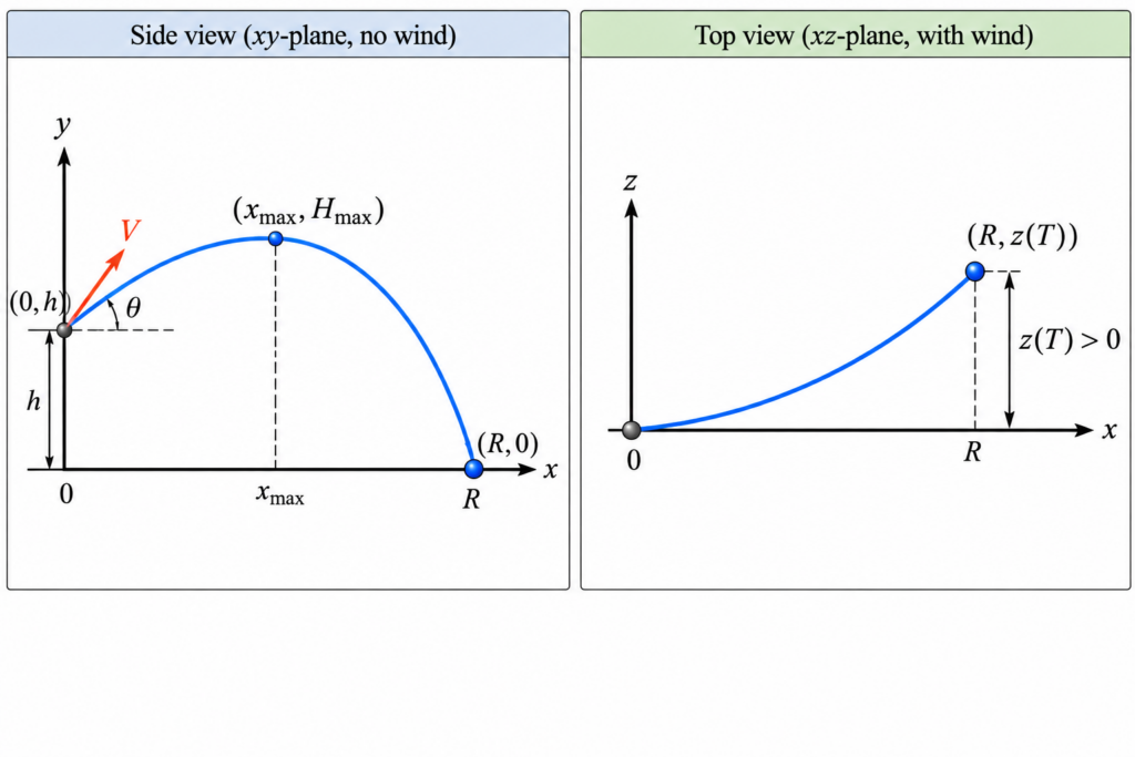
    The standard projectile-motion problem is familiar from calculus and physics: a projectile is launched with initial speed V at an angle θ above the horizontal from an initial height h. Gravity pulls it downward, and we ask two basic questions:

    • How high does the projectile go?
    • How far does it travel before hitting the ground?

    But real projectiles do not necessarily stay in a vertical plane. What happens if we add a horizontal wind blowing from the side? And what happens if we also include air resistance?

    The familiar two-dimensional parabola becomes a genuinely three-dimensional trajectory. With a simple model of air resistance, we can still obtain explicit formulas for almost everything.

    1. Setting Up the Coordinates

    Choose coordinates so that:

    • x is the original horizontal firing direction,
    • y is the vertical direction,
    • z is the sideways horizontal direction.

    The projectile is fired in the vertical xy-plane, so initially there is no velocity in the z-direction.

    The initial position is

    r (0) = ( 0,h,0 ).

    The initial velocity is

    v (0) = ( V⁢cos⁡θ , V⁢sin⁡θ ,0 ).

    2. Adding Wind

    Suppose a horizontal wind has speed W and makes an angle φ with the positive x-direction. Its velocity vector is

    w= ( W⁢cos⁡φ ,0, W⁢sin⁡φ ).

    The component W⁢cos⁡φ pushes along the original firing direction, while W⁢sin⁡φ produces sideways motion.

    3. Air Resistance Must Be Relative to the Air

    If there were no air resistance, a steady wind would have no effect on an ideal point projectile. Wind matters because the projectile interacts with the surrounding air.

    For a simple model, assume that air resistance is proportional to the projectile’s velocity relative to the moving air. If k is the drag constant per unit mass, the acceleration due to air resistance is

    −k ( v − w ).

    Gravity contributes

    ( 0,−g,0 ).

    Therefore the equation of motion is

    r″ = −gj −k ( r′ − w ).

    4. Three Differential Equations

    Writing the vector equation component by component gives

    x″ = −k ( x′ − W⁢cos⁡φ ) y″ = −g −ky′ z″ = −k ( z′ − W⁢sin⁡φ ).

    Although the trajectory is three-dimensional, something very convenient has happened: the three equations can be solved separately.

    5. Solving for the Velocity

    The velocity in the x-direction is

    vx (t) = W⁢cos⁡φ + ( V⁢cos⁡θ − W⁢cos⁡φ ) e−kt.

    The sideways velocity is

    vz (t) = W⁢sin⁡φ ( 1− e−kt ).

    The vertical velocity is

    vy (t) = ( V⁢sin⁡θ + gk ) e−kt − gk.

    Notice the long-term behavior. The horizontal velocity approaches the wind velocity, while the vertical velocity approaches

    −gk.

    In this linear-drag model, this is the terminal vertical velocity.

    6. The 3D Position

    Integrating the velocity components and using the initial position gives

    x (t) = W⁢cos⁡φt + V⁢cos⁡θ − W⁢cos⁡φ k ( 1− e−kt ). y (t) = h − gkt + V⁢sin⁡θ +gk k ( 1− e−kt ). z (t) = W⁢sin⁡φ [ t − 1− e−kt k ].

    These three equations describe the complete trajectory through space. Unlike the usual projectile trajectory, this curve is not a parabola.

    7. When Does the Projectile Reach Its Maximum Height?

    At maximum height the vertical velocity is zero:

    vy ( tmax ) =0.

    Therefore

    ( V⁢sin⁡θ +gk ) e −ktmax = gk.

    Solving for time gives

    tmax = 1k ln⁡ ( 1 + kV⁢sin⁡θ g ).

    8. Maximum Height

    Substituting this time into the vertical position formula and simplifying gives

    Hmax = h + V⁢sin⁡θ k − gk2 ln⁡ ( 1 + kV⁢sin⁡θ g ).

    An interesting consequence is that the horizontal wind does not appear in this formula. In this model, horizontal wind changes where the projectile lands, but it does not change its maximum height.

    9. When Does It Hit the Ground?

    Let T denote the time at which the projectile hits the ground. We find T by setting

    y (T) =0.

    Thus T satisfies

    h − gkT + V⁢sin⁡θ + gk k ( 1− e−kT ) =0.

    Here we encounter an important difference from the standard projectile problem. Without air resistance, finding the flight time requires solving a quadratic equation. With linear air resistance, the unknown T appears both outside and inside an exponential.

    In practice, the positive solution can be found numerically using a calculator, computer, graphing program, or Newton’s method.

    10. Where Does It Land?

    Once the flight time T has been found, the landing point is

    ( x(T) , 0 , z(T) ).

    The downrange distance in the original firing direction is x(T) , while the sideways displacement is z(T) .

    The total horizontal distance between the launch point and landing point is

    R= x(T) 2 + z(T) 2 .

    So in three dimensions, the question “How far does the projectile go?” has more than one possible answer. We can ask for its downrange distance, its sideways drift, or its total horizontal displacement.

    11. How Far Sideways Does the Wind Push It?

    The sideways displacement at landing is

    z (T) = W⁢sin⁡φ [ T − 1− e−kT k ].

    This is zero when the wind blows exactly along the original firing direction. It becomes nonzero when the wind has a crosswind component.

    12. A Consistency Check: Remove Air Resistance

    A good mathematical model should reproduce the familiar result when the new effect is removed. Let the drag coefficient k approach zero. A key limit is

    lim k→0 1− e−kt k =t.

    As air resistance disappears, the vertical motion approaches

    y (t) = h + V⁢sin⁡θt − 12 gt2,

    which is exactly the standard projectile-motion formula.

    The maximum-height formula also approaches

    Hmax → h + V2 sin⁡θ 2 2g .

    Again, this is precisely the familiar result.

    13. From a Parabola to a Space Curve

    The ordinary projectile problem is two-dimensional. Its trajectory is a parabola contained in a vertical plane.

    Adding a crosswind and air resistance changes the geometry completely. The projectile now moves simultaneously forward, vertically, and sideways. Its position is described parametrically by

    r (t) = ( x(t) , y(t) , z(t) ).

    This is a natural example of why parametric vector equations are useful: there is no need to force a three-dimensional trajectory into a single equation involving x, y, and z.

    14. What Makes This Problem Interesting?

    The standard projectile problem is often presented as an application of quadratic functions. But a relatively small change in the physical assumptions leads to much richer mathematics.

    The three-dimensional model combines:

    • vectors and parametric curves,
    • differential equations,
    • exponential functions,
    • optimization,
    • numerical root finding,
    • limits,
    • and mathematical modeling.

    Most importantly, the model separates two questions that look similar but are physically different. Gravity and vertical drag determine when the projectile hits the ground. The wind and horizontal drag then determine where it lands.

    That is the real advantage of moving from the familiar two-dimensional projectile problem to a three-dimensional model: instead of asking only “How far?”, we can ask the more interesting question: Where will it land?
    Worked Example: Where Does the Projectile Land?

    Let us use the formulas above with actual numbers. Suppose a projectile is launched from a height of 10 meters with an initial speed of 40 m/s at an angle of 45° above the horizontal.

    A horizontal wind blows at 10 m/s at an angle of 60° from the original firing direction. Assume a linear drag constant k = 0.10 s−1 and take g = 9.81 m/s2.

    Thus our data are

    h=10 m,   V=40 m/s,   θ=45°, W=10 m/s,   φ=60°,   k=0.10 s −1.

    Step 1: When Does It Reach Maximum Height?

    The time at which the projectile reaches its maximum height is

    tmax = 1k ln⁡ ( 1 + kV ⁢ sin⁡θ g ).

    Substituting the numerical values gives

    tmax = 10.10 ln⁡ ( 1 + ( 0.10 ) ( 40 ) sin⁡ 45° 9.81 ).

    Therefore,

    tmax ≈ 2.533 s.

    The projectile reaches its highest point about 2.53 seconds after launch.

    Step 2: What Is the Maximum Height?

    The maximum height is

    Hmax = h + V ⁢ sin⁡θ k − g k2 ln⁡ ( 1 + kV ⁢ sin⁡θ g ).

    Substitution gives

    Hmax = 10 + 40 sin⁡ 45° 0.10 − 9.81 0.102 ln⁡ ( 1 + ( 0.10 ) ( 40 ) sin⁡ 45° 9.81 ).

    Thus

    Hmax ≈ 44.32 m.

    The projectile rises to approximately 44.32 meters above the ground.

    Step 3: When Does It Hit the Ground?

    The projectile hits the ground when y ( T ) =0 . For our values, this means solving

    10 − 9.810.10T + 40 sin⁡ 45° + 9.810.10 0.10 ( 1 − e −0.10T ) =0.

    Unlike the standard projectile problem, this is not a quadratic equation. The unknown T appears both by itself and in an exponential. Solving the equation numerically gives

    T ≈ 5.698 s.

    So the projectile is in the air for approximately 5.70 seconds.

    Step 4: How Far Downrange Does It Travel?

    The horizontal x-coordinate at landing is

    x ( T ) = W ⁢ cos⁡φ ⁢T + V ⁢ cos⁡θ − W ⁢ cos⁡φ k ( 1 − e −kT ).

    Substituting T≈5.698 gives

    x ( T ) ≈ 129.62 m.

    Thus the projectile travels approximately 129.62 meters downrange.

    Step 5: How Far Sideways Does the Wind Push It?

    The sideways coordinate at landing is

    z ( T ) = W ⁢ sin⁡φ [ T − 1 − e −kT k ].

    Substituting the numerical values gives

    z ( T ) = 10 sin⁡ 60° [ 5.698 − 1 − e − ( 0.10 ) ( 5.698 ) 0.10 ].

    Therefore,

    z ( T ) ≈ 11.73 m.

    The wind has pushed the projectile approximately 11.73 meters sideways from the original vertical firing plane.

    Step 6: Where Does It Land?

    We now know both horizontal coordinates. Therefore the landing point is approximately

    P = ( 129.62 , 0 , 11.73 ) m.

    In other words, the projectile lands approximately 129.62 meters downrange and 11.73 meters sideways from the original vertical firing plane.

    Step 7: Total Horizontal Displacement

    The straight-line horizontal distance from the point directly below the launch position to the landing point is

    R = x ( T ) 2 + z ( T ) 2 .

    Therefore,

    R = 129.622 + 11.732 ≈ 130.15 m.

    The Answer

    For this example, the projectile reaches a maximum height of approximately 44.32 m and stays in the air for approximately 5.70 s.

    It lands approximately 129.62 m downrange and 11.73 m sideways from the original vertical firing plane. Thus its landing point is

    ( 129.62 , 0 , 11.73 ) m.

    The total horizontal displacement from the point directly below the launch position is approximately 130.15 m. The sideways displacement shows exactly how the wind changes the familiar two-dimensional projectile problem into a three-dimensional one.


    For another example of how calculus can reveal something unexpected in a real-world motion problem, see Sliding Ladder: Is It Better to Slide or Jump?.

    Projectile motion and planetary motion are both governed by Newton’s laws. Near Earth’s surface, gravity is approximately constant, while planetary orbits require the inverse-square law of gravitation. Explore this connection in Kepler’s Laws: How Calculus Explains Planetary Motion .
  • A Sliding Ladder: Is It Better to Slide or Jump?

    The sliding-ladder problem is one of the most familiar examples of related rates in calculus.

    A ladder leans against a vertical wall. The bottom begins to slide away from the wall, while the top slides downward.

    Usually the textbook asks:

    How fast is the top of the ladder moving?

    But there is a more interesting question:

    If you were on the ladder when it started to slide, what would the mathematics predict as the ladder approached the floor?

    The answer is surprising.

    The Geometry

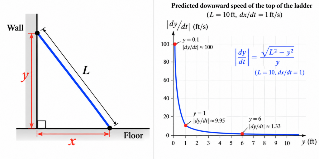
    Suppose the ladder has fixed length L. Let x be the distance from the bottom of the ladder to the wall, and let y be the height of the top of the ladder above the floor.

    Because the ladder, wall, and floor form a right triangle,

    x2 + y2 = L2 .

    As the ladder slides, both x and y change with time. Differentiate with respect to t:

    2x dx dt + 2y dy dt = 0 .

    Dividing by 2 gives

    x dx dt + y dy dt = 0 .

    Therefore,

    dy dt = − xy dx dt .

    This is the standard related-rates formula for a sliding ladder.

    Suppose the Bottom Moves at Constant Speed

    Assume that the bottom of the ladder moves away from the wall at a constant speed v:

    dx dt = v , v>0 .

    Then

    dy dt = − v xy .

    Since

    x = L2 − y2 ,

    we can also write

    dy dt = − v L2 − y2 y .

    The minus sign tells us that the top of the ladder is moving downward.

    What Happens Near the Floor?

    As the top of the ladder approaches the floor,

    y → 0+ , x → L .

    Therefore,

    xy → ∞ ,

    and consequently

    dy dt → −∞ .

    According to this model, the top of the ladder moves downward faster and faster, and its vertical speed becomes arbitrarily large as it approaches the floor.

    A Numerical Example

    Suppose the ladder is 10 feet long and its bottom slides away from the wall at

    dx dt = 1 ft/s .

    When the top is 6 feet above the floor,

    x = 100−36 = 8 .

    Thus,

    dy dt = − 86 = − 43 ft/s .

    Nothing dramatic yet. But when the top is only 1 foot above the floor,

    x = 99 ,

    so

    dy dt = −99 ≈ −9.95 ft/s .

    When the top is only 0.1 foot above the floor,

    dy dt = − 99.99 0.1 ≈ −100 ft/s .

    The closer the top gets to the floor, the larger the predicted downward speed becomes.

    What About dy/dx?

    There is another way to see where this strange behavior comes from. Differentiate

    x2 + y2 = L2

    with respect to x. We obtain

    2x + 2y dy dx = 0 ,

    and therefore

    dy dx = − xy .

    As the ladder approaches the floor,

    dy dx → −∞ .

    Geometrically, this makes sense. The point (x,y) moves along the quarter-circle

    x2 + y2 = L2 ,

    which has a vertical tangent at (L,0) .

    But there is an important distinction: dy/dx is not a velocity.

    The connection with velocity is

    dy dt = dy dx dx dt .

    If the horizontal speed remains positive and constant while dy dx becomes unbounded, then the predicted vertical velocity becomes unbounded as well.

    So Is It Better to Slide or Jump?

    At first sight, the mathematics seems to give a disturbing answer. If you remain with the ladder, the simple model predicts that the downward speed can become enormous near the floor.

    Does that mean you should jump?

    Not so fast.

    The calculation has actually revealed something more interesting: the mathematical model has become physically unrealistic.

    We assumed that the bottom of the ladder continues moving horizontally at a constant speed all the way until the ladder becomes horizontal. A real ladder cannot behave this way.

    A real ladder has mass and rotational inertia. There is friction between the ladder and the floor and between the ladder and the wall. The ladder may lose contact with the wall. A person standing on it changes the center of mass and the forces acting on the system.

    Most importantly, a real physical system cannot produce the infinite vertical velocity predicted by this simplified model.

    So the infinity does not tell us that a real person will hit the floor at infinite speed.

    It tells us that one of our assumptions must fail before that happens.

    Calculus as a Warning About a Model

    This is what makes the sliding-ladder problem more interesting than the usual textbook exercise.

    Related rates correctly tells us that

    dy dt = − xy dx dt .

    Under the additional assumption that the horizontal speed stays constant, it follows that

    | dy dt | → ∞ .

    The calculus is not wrong. The assumption is unrealistic.

    When a correct calculation produces a physically impossible result, the mathematics may be telling us where our model stops being valid.

    The humble sliding-ladder problem is therefore not just an exercise in implicit differentiation. It is also a lesson about the difference between mathematics and the physical world.


    Related: Another example of mathematics revealing the limitations of a model is Population Growth: From Exponential Growth to the Logistic Equation .


    For another example of how calculus models motion in the real world, see Projectile Motion in 3D: Adding Wind and Air Resistance, where the standard projectile problem is extended to include wind and air resistance.

    Another classical motion problem with a surprising answer is the brachistochrone problem. The fastest path is a cycloid when there is no resistance—but what happens when fluid resistance is added?

    Calculus describes many kinds of motion, from mechanical systems on Earth to planets orbiting the Sun. For a fascinating application of derivatives, geometry, and Newton’s laws, read Kepler’s Laws: How Calculus Explains Planetary Motion .
  • The Population Model That Fails—and Why Its Equation Is Everywhere: Population, Interest, and Radioactive Decay

    “`html

    A remarkably simple differential equation appears in many different places in the real world. We will begin with population growth. The first model we try will have a serious problem: it predicts unlimited growth. Fixing that problem will lead us to the logistic equation.

    Then, surprisingly, we will return to our original equation and discover that it was not a bad equation at all. The same equation describes continuous compound interest, radioactive decay, and many other processes.

    1. The Simplest Population Model

    Let P(t) denote a population at time t.

    One of the simplest assumptions we can make is this: the rate at which the population grows is proportional to the population itself.

    dP dt = kP, P(0) = P0.

    Here k>0 is a constant. The idea seems reasonable. If there are twice as many individuals, we might expect approximately twice as many births. A larger population therefore grows faster.

    The equation is separable:

    dPP = kdt.

    Integrating gives

    lnP = kt+C,

    and therefore

    P(t) = P0 ekt.

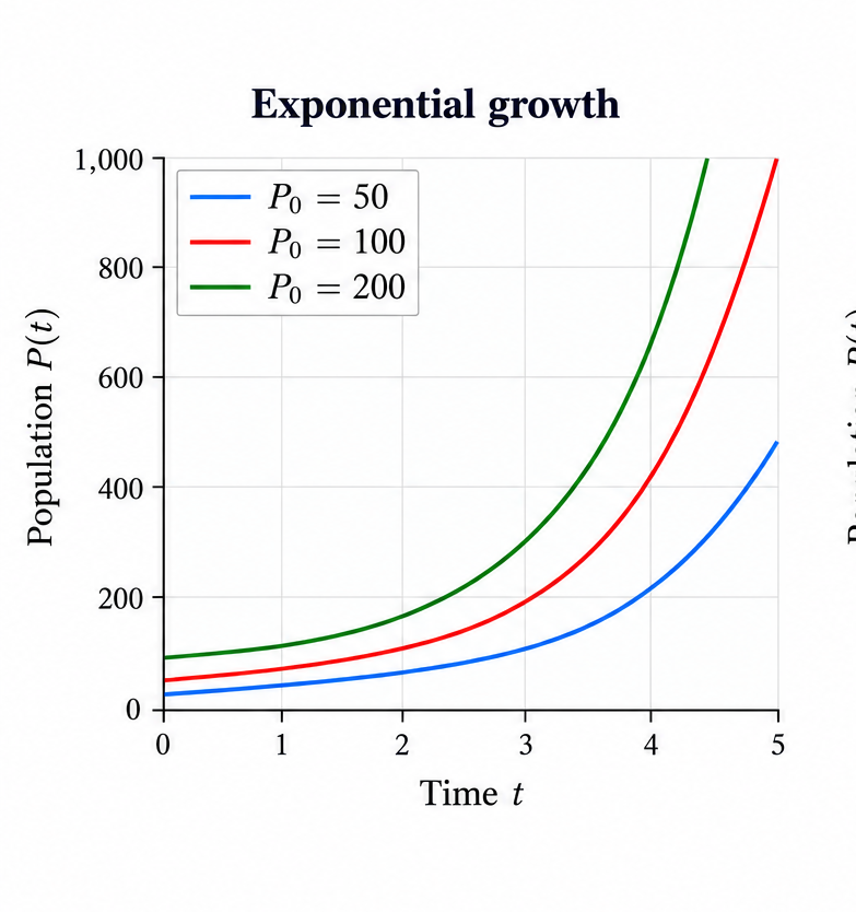
    This is exponential growth.

    There is an immediate problem. If k>0, then

    P(t) → ∞ as t→∞.

    According to this model, the population eventually becomes arbitrarily large. That cannot continue indefinitely in the real world. Food, water, space, and other resources are limited.

    So our first population model is useful for describing growth over some periods, but it cannot be the whole story.

    “`
    “`html

    2. Introducing a Carrying Capacity

    Suppose the environment can sustainably support a maximum population K. This number is called the carrying capacity.

    We modify our original equation to

    dP dt = kP ( 1 − P K )

    This is the logistic equation.

    The new factor

    ( 1 − P K )

    is what changes everything. When the population is small compared with K, this factor is close to 1, so the population behaves approximately like ordinary exponential growth. As the population becomes larger, the factor becomes smaller and the growth slows down.

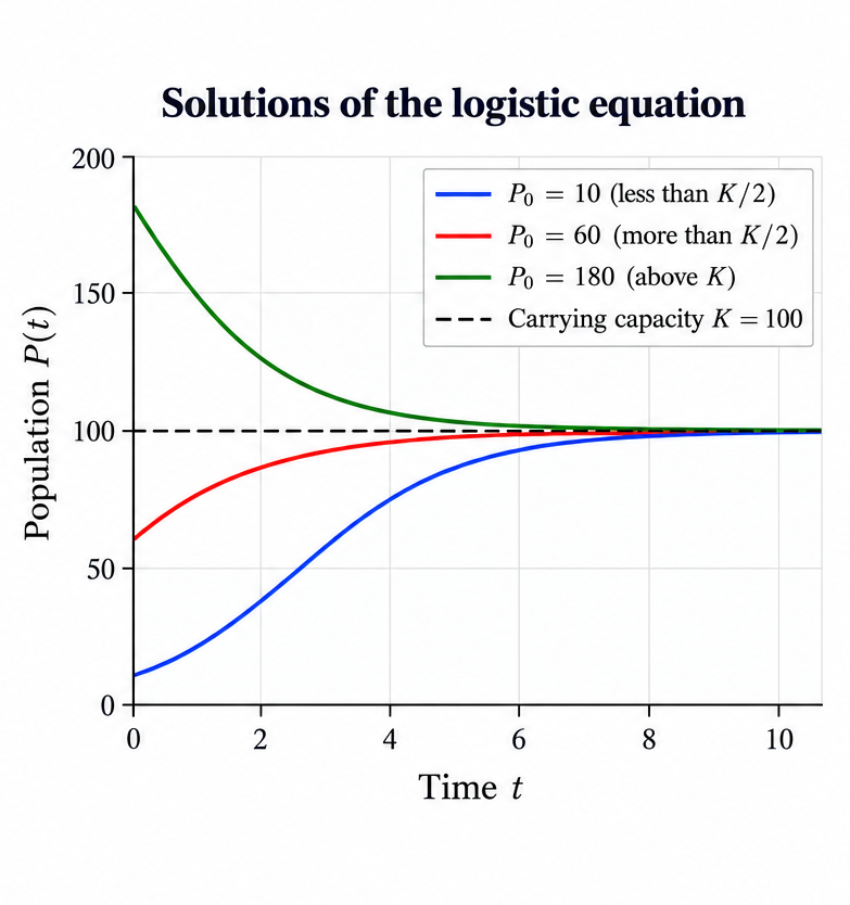
    We Can Predict the Solutions Without Solving the Equation

    This is one of the most useful ideas in differential equations: we do not always need an explicit formula to understand what the solutions will do.

    First suppose

    0 < P < K.

    Then

    ( 1 − P K ) > 0,

    and consequently

    dP dt > 0.

    So the population increases.

    Now suppose P=K. Then

    ( 1 − P K ) = 0,

    so

    dP dt = 0.

    The population remains constant at the carrying capacity.

    Finally, if P>K, then

    ( 1 − P K ) < 0,

    and therefore

    dP dt < 0.

    The population decreases toward the carrying capacity.

    Where Is the Population Growing Fastest?

    The growth rate is

    kP ( 1 − P K ).

    As a function of P, this is a downward-opening quadratic:

    kP − kP2 K .

    Its maximum occurs at

    P = K 2 .

    This tells us something important about the shape of the population curve.

    If P0 < K2 , the population initially grows faster and faster. When it reaches P = K2 , its growth rate is greatest. After that, the population continues to increase, but more and more slowly as it approaches K. This produces the familiar S-shaped logistic curve.

    If K2 < P0 < K , the population begins above the point of fastest growth. It still increases toward K, but it slows down from the beginning.

    Finally, if P0 > K , the population decreases toward K.

    Thus, before solving the logistic equation, we can already predict the three different types of solution curves shown in the next figure.

    “`
    “`html id=”p87fcf”

    3. Now Let Us Solve the Logistic Equation

    We now return to the logistic equation

    dP dt = kP ( 1 − P K ), P(0) = P0.

    We have already learned a great deal about its solutions without solving it. Now let us find the actual formula.

    First separate the variables:

    dP P ( 1 − P K ) = kdt.

    Since

    1 P ( 1 − P K ) = 1P + 1 K−P ,

    we can integrate:

    ∫ ( 1P + 1 K−P ) dP = ∫ kdt.

    This gives

    lnP − ln ( K−P ) = kt + C.

    Combining the logarithms,

    ln ( P K−P ) = kt + C.

    Exponentiating both sides gives

    P K−P = C e kt .

    Using the initial condition P(0) = P0 , we obtain

    C = P0 K − P0 .

    After solving for P, we obtain the logistic growth formula:

    P(t) = K 1 + K − P0 P0 e −kt .

    Now the formula confirms what we predicted from the differential equation. For positive initial populations, the population approaches the carrying capacity:

    P(t) → K as t→∞.

    So the carrying capacity is not merely a number inserted into the model. It becomes the long-term population predicted by the model.

    4. Was Our Original Equation Really So Bad?

    We rejected the equation

    dy dt = ky

    as a model of population growth over an unlimited period of time. But the equation itself is one of the most important differential equations in mathematics.

    The initial-value problem

    dy dt = ky, y(0) = y0

    has the solution

    y(t) = y0 e kt .

    What changes from one application to another is the meaning of y and the sign and meaning of the proportionality constant.

    5. Continuous Compound Interest

    Suppose an amount of money A(t) earns interest continuously at an annual rate r. The rate at which the account balance changes is proportional to the amount currently in the account:

    dA dt = rA, A(0) = A0.

    Therefore,

    A(t) = A0 e rt .

    The same equation that produced exponential population growth now describes the growth of money.

    6. Radioactive Decay

    Now consider a radioactive substance. The more radioactive nuclei that are present, the more nuclei are available to decay. Thus, the magnitude of the decay rate is proportional to the amount currently present.

    This time the quantity is decreasing, so we write

    dN dt = − λN, N(0) = N0,

    where λ>0 is the decay constant.

    The solution is

    N(t) = N0 e − λt .

    7. One Equation, Many Processes

    We began with perhaps the simplest population model imaginable: the rate of change of a population is proportional to the population itself.

    As a long-term population model, it failed. Unlimited exponential population growth is impossible in an environment with limited resources.

    Introducing a carrying capacity led naturally to the logistic equation. Even more importantly, we were able to predict the behavior of its solutions before solving the equation.

    But our original equation was far from useless. The same basic mathematical law appears in continuous compound interest and radioactive decay.

    The common idea is simple:

    The rate of change of a quantity is proportional to the amount of that quantity currently present.

    Population, money, and radioactive atoms seem like completely different things. Mathematically, however, they can obey the same law.

    That is one of the remarkable features of differential equations: the same mathematical equation can describe very different processes in the real world.


    Related: See another example where a simple mathematical model produces a surprising—and ultimately unrealistic—prediction: A Sliding Ladder: Is It Better to Slide or Jump? .