Elite Math Program

Tag: infinite series

How the Ancient Greeks Summed Infinite Series Without Calculus
Can infinitely many pieces have a finite total area? The Greeks approached this question through geometric exhaustion. Archimedes proved that a parabolic segment has four-thirds the area of its largest inscribed triangle. Here we explain the geometry with modern notation, clearly distinguishing ancient arguments from modern illustrations.

1. Zeno and infinitely many steps

Travel half a unit, then a quarter, then an eighth, and so on. The infinite subdivision raises Zeno’s famous question: can infinitely many stages have a finite total?
12+14+18+⋯=1
Figure 1. Zeno’s successive halfway distances. This is a modern diagram of the ancient philosophical problem.

After n steps the distance left is 1/2ⁿ. It tends to zero, although no finite step reaches the endpoint.

2. A square proves a geometric series

Partition a unit square into vertical strips of widths 1/2, 1/4, 1/8, … . The strip areas have exactly these values.

Figure 2. Successive strips fill the unit square in the limit. Each new strip is half the remaining width.
Sn=1−12n
Since the unfilled strip has area 1/2ⁿ, its area approaches zero. The same argument gives the general geometric sum when 0 < q < 1:
1+q+q2+⋯=11−q
The colored-square construction and modern series notation are teaching devices, not a reconstruction of a particular surviving ancient proof.

3. Archimedes’ quadrature of the parabola

Consider the region between y = 1 − x² and the chord from (−1,0) to (1,0). Its largest inscribed triangle has vertices (−1,0), (0,1), (1,0), and area T = 1.

Figure 3. The blue triangle has area T. The orange pair totals T/4, and the green group totals T/16. Later generations continue the same pattern.

Why does every generation shrink by a factor of four?

The next triangle on the left has vertices (−1,0), (0,1), and (−1/2,3/4). The determinant formula gives area 1/8. The symmetric right triangle also has area 1/8, so their combined area is T/4.

For any two points of the parabola with x-coordinates a and b, the tangent parallel to their chord occurs at x = (a+b)/2. A determinant calculation gives the inscribed triangle area:
T(a,b)=b−a38
Halving the interval [a,b] produces two child triangles, each with 1/8 of its parent’s area. Thus their combined area is 1/4 of the parent’s area. This repeats at every stage.
A=T(1+14+116+⋯)=4T3
Since T = 1 in our example, the curved segment has area 4/3. Modern integration confirms that the integral of 1 − x² from −1 to 1 equals 4/3.

4. Why exhaustion proves the result

Archimedes needed more than an attractive pattern: he had to show that the remaining curved slivers could have arbitrarily small total area. Let S_n denote the first n+1 generations. The finite geometric sum is
Sn=4T3(1−14n+1)
Each remaining parabolic segment fits inside a parallelogram of twice the area of its largest inscribed triangle. Thus, after n generations, the total leftover area R_n obeys:
0≤Rn≤2T4n+1
The right side tends to zero, proving that the triangles exhaust the parabolic segment. This is a modern remainder-bound presentation of the geometric reasoning.

Figure 4. The finite areas approach 4T/3 while the leftover area becomes arbitrarily small. Schematic, not to scale.

5. Another area series: thirds

A rectangle of area 1/2 can be partitioned into strips with areas 1/3, 1/9, 1/27, … by taking two-thirds of what remains at each step. Hence
13+19+127+⋯=12
6. Why the harmonic series behaves differently

Not every infinite collection of positive areas has a finite sum. Group the harmonic series as 1; 1/2; (1/3 + 1/4); (1/5 + ⋯ + 1/8); and so on. Every group after the first totals at least 1/2. Thus the partial sums grow without bound. Rectangles of width 1 and heights 1, 1/2, 1/3, … have unbounded combined area.

7. From Greek geometry to calculus

The method of exhaustion anticipates integration: approximate a curved region with simple shapes, then control the error. The Greeks did not write modern limit or integral notation, but their finite geometric comparisons could establish exact areas.

Discovery problems

1. Give a geometric proof that 1/3 + 1/9 + 1/27 + ⋯ = 1/2.

2. For a starting triangle of area T, find the sum of the first n+1 Archimedean generations and bound the remainder.

3. For the segment under y = 9 − x² above the x-axis, find the largest inscribed triangle area and then the curved area. Check by integration.

4. Show geometrically by grouping that the harmonic series diverges, and explain why this does not contradict the square partition.

Solutions (click to reveal)

Solution 1
Begin with a rectangle of area 1/2. Take two-thirds of its area, then two-thirds of the remainder, repeatedly. The removed areas are 1/3, 1/9, 1/27, … . The remainder after n steps is (1/2)(1/3)ⁿ, which tends to zero.

Solution 2
S_n = (4T/3)(1 − 4⁻⁽ⁿ⁺¹⁾). The unfilled area is at most 2T/4ⁿ⁺¹, by the enclosing-parallelogram bound. It tends to zero.

Solution 3
The endpoints are (−3,0), (3,0) and the apex is (0,9). The triangle area is T = (1/2)(6)(9) = 27. Archimedes gives 4T/3 = 36. Integrating 9 − x² from −3 to 3 also gives 36.

Solution 4
Group 1/2; (1/3+1/4); (1/5+⋯+1/8); and so on. Every group contains twice as many terms as the previous, each at least half the preceding minimum, so each group totals at least 1/2. The area grows without bound, unlike the square partition whose total is at most 1.

Historical sources
- Archimedes, Quadrature of the Parabola, especially Propositions 21–24.
- Euclid, Elements, Book XII.
- Thomas L. Heath, The Works of Archimedes (1897 translation and commentary).
Historical note: The modern algebra, colored diagrams, and integration checks are explanatory additions, not verbatim ancient arguments.
Archimedes used geometry to evaluate infinite sums long before the development of calculus. Centuries later, mathematicians discovered remarkable geometric and analytic methods for evaluating more complicated series. Explore one such example in our article on the Basel problem and its solution using a double integral .

The relationship between infinity and geometry continues to produce surprising results. For example, a surface can have infinite area while enclosing a finite volume. Discover this phenomenon in Gabriel’s Horn .
October 7, 2026
Can a Function Be Continuous Everywhere but Differentiable Nowhere?

A basic theorem from calculus says that every differentiable function is continuous. But what about the converse?

If a function is continuous everywhere, must it be differentiable somewhere?

It seems reasonable. A continuous graph has no jumps or breaks, and we might expect that if we zoom in far enough, at least some part of the graph should begin to look like a straight line.

Surprisingly, this intuition is completely wrong.

There are functions that are continuous at every point and yet differentiable at no point.

Continuous Does Not Mean Smooth

We learn early in calculus that

$differentiable ⟹ continuous.$

The reverse implication is false. Continuity only says that nearby inputs give nearby outputs. It does not say that the graph must have a well-defined tangent line.

A corner such as the one in the graph of $f (x) = | x |$ already shows that a continuous function can fail to be differentiable at a point.

But that raises a much more surprising question:

Can a continuous function have a corner-like failure of smoothness everywhere?

Weierstrass’s Remarkable Example

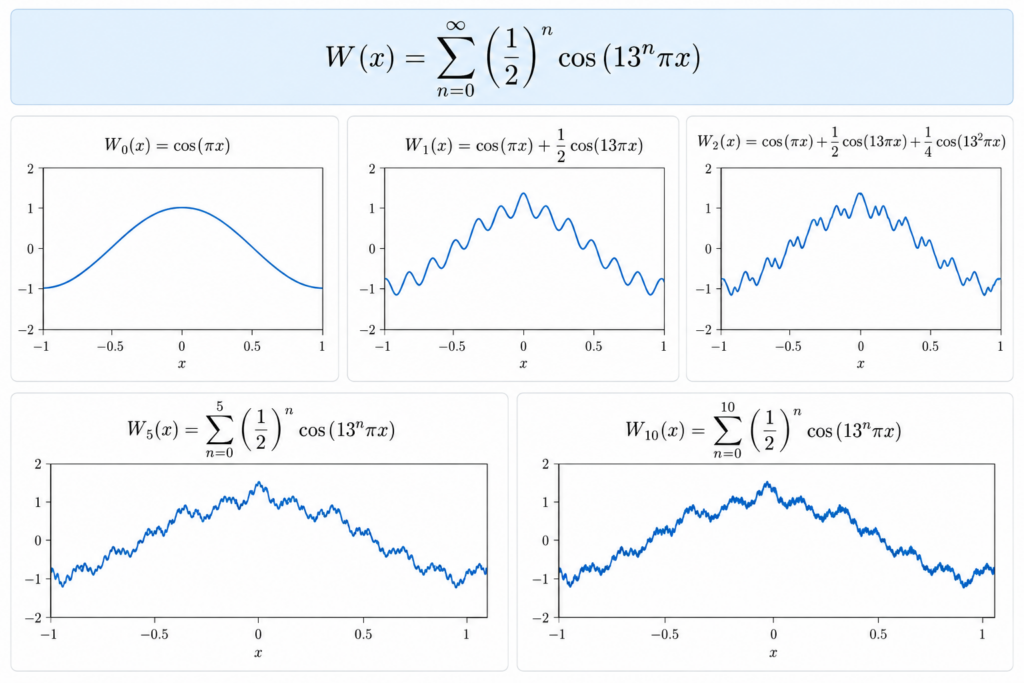
A famous example is the Weierstrass function, constructed from an infinite sum of cosine waves:

$W (x) = \sum_{n = 0}^{\infty} a^{n} \cos (b^{n} π x) .$

Here $0 < a < 1$ and $b$ is chosen sufficiently large.

For a concrete example, take

$a = \frac{1}{2}, b = 13 .$

Then

$W (x) = \sum_{n = 0}^{\infty} \frac{1}{2^{n}} \cos (13^{n} π x) .$

What Is Happening?

Look carefully at the two competing parts of each term.

The amplitude is

$a^{n} .$

Because $0 < a < 1,$ these amplitudes become smaller and smaller.

But the frequency is controlled by

$b^{n},$

which becomes larger and larger.

So every new term adds a smaller wave—but a wave that oscillates much more rapidly than the waves before it.

Watch the Roughness Appear

Instead of looking immediately at the infinite sum, consider its partial sums

$W_{N} (x) = \sum_{n = 0}^{N} a^{n} \cos (b^{n} π x) .$

The first term is just a smooth cosine curve. Adding more terms creates smaller and faster oscillations. The graph becomes increasingly rough.

Every finite partial sum is still perfectly smooth. The strange behavior appears only in the limit as infinitely many increasingly rapid oscillations are added.

Why Is the Function Continuous?

The continuity is actually the easier part. Since

$| a^{n} \cos (b^{n} π x) | \leq a^{n},$

and the geometric series

$\sum_{n = 0}^{\infty} a^{n} = \frac{1}{1 - a}$

converges, the Weierstrass series converges uniformly. Each partial sum is continuous, and a uniform limit of continuous functions is continuous.

Thus $W (x)$ is continuous everywhere.

So Why Is It Not Differentiable?

Here is the intuition.

At any fixed scale, the graph may appear almost smooth. But when we zoom in, terms with higher frequencies become visible. Zoom in again, and still higher-frequency terms reveal another layer of oscillation.

There is no scale at which the graph finally settles down into a straight line.

A derivative would require the difference quotient

$\frac{W (x + h) - W (x)}{h}$

to approach a single finite value as $h \to 0 .$ For suitable choices of $a$ and $b,$ the increasingly rapid oscillations prevent this from happening at every point.

A rigorous proof of nowhere differentiability requires more work, but the mechanism is visible directly in the construction: decreasing amplitudes preserve continuity while rapidly increasing frequencies destroy local smoothness.

A Change in Mathematical Intuition

Examples like the Weierstrass function were historically important because they challenged the idea that a continuous curve should be smooth except perhaps at a few exceptional points.

Continuity turns out to permit behavior far more complicated than our geometric intuition initially suggests.

A function can have no jumps, no breaks, and no discontinuities anywhere—and still have no tangent line anywhere.

The Main Surprise

The Weierstrass function separates two ideas that can look almost identical when we first learn calculus:

continuity and smoothness are not the same thing.

Even more remarkably, the failure of smoothness does not have to occur at a few isolated points. It can occur at every single point.

Continue exploring: Continuous functions can behave strangely in other ways too. Can a Curve Fill a Square? The Mathematics of Space-Filling Curves

October 2, 2026
How Newton Computed Sines and Cosines Without a Calculator

Today, if we want to know the sine or cosine of an angle, we simply press a button on a calculator. But suppose there is no calculator, no computer, and no trigonometric table.

How could we actually compute, for example,
$\sin (1 °)$
using only arithmetic?

One answer comes from the classical sine and cosine series associated with Isaac Newton. The series appeared in Newton’s De analysi per aequationes numero terminorum infinitas, written in 1665–1666. The elegant derivation below follows a later mean-value approach presented by Heinrich Dörrie, written here in modern calculus notation.

The goal

We want formulas that allow us to calculate the sine and cosine of an angle x. The angle must be measured in radians.

The formulas we will obtain are
$\sin x = x - \frac{x^{3}}{3!} + \frac{x^{5}}{5!} - \frac{x^{7}}{7!} + \dots$
and
$\cos x = 1 - \frac{x^{2}}{2!} + \frac{x^{4}}{4!} - \frac{x^{6}}{6!} + \dots$
Today these are familiar power series. What is especially interesting is that we can derive them from a very simple idea: repeatedly taking averages.

The key idea: average values

Consider the average value of the sine function on the interval from 0 to x. In modern calculus notation,
$\frac{1}{x} \int_{0}^{x} \sin t d t = \frac{1 - \cos x}{x}$
Similarly, the average value of cosine is
$\frac{1}{x} \int_{0}^{x} \cos t d t = \frac{\sin x}{x}$
These two elementary formulas are enough to generate increasingly accurate approximations for both sine and cosine.

Start with the simplest inequality

For a positive angle x sufficiently close to zero,
$\cos x < 1$
Now take the average of both sides from 0 to x. The average of the left side is
$\frac{\sin x}{x}$
while the average of 1 is simply 1. Therefore,
$\frac{\sin x}{x} < 1$
and hence
$\sin x < x$
We have obtained our first approximation:
$\sin x \approx x$
Average again

Now start with
$\sin x < x$
and take averages once more. The average of the left side is
$\frac{1 - \cos x}{x}$
while the average of the function t on the interval from 0 to x is x/2. Thus,
$\frac{1 - \cos x}{x} < \frac{x}{2}$
Multiplying by x and rearranging gives
$\cos x > 1 - \frac{x^{2}}{2!}$
And again

Take averages of this new inequality. The average of cosine is
$\frac{\sin x}{x}$
and the average of the right-hand side is
$1 - \frac{x^{2}}{6}$
Therefore,
$\frac{\sin x}{x} > 1 - \frac{x^{2}}{6}$
and consequently
$\sin x > x - \frac{x^{3}}{3!}$
We have now trapped sine between two simple expressions:
$x - \frac{x^{3}}{3!} < \sin x < x$
Keep repeating the process

Each time we take another average, we obtain another term. Continuing gives alternating upper and lower bounds:
$\sin x < x - \frac{x^{3}}{3!} + \frac{x^{5}}{5!}$
and then
$\sin x > x - \frac{x^{3}}{3!} + \frac{x^{5}}{5!} - \frac{x^{7}}{7!}$
The upper and lower approximations become closer and closer. Their common limiting value gives
$\sin x = x - \frac{x^{3}}{3!} + \frac{x^{5}}{5!} - \frac{x^{7}}{7!} + \dots$
The same procedure gives
$\cos x = 1 - \frac{x^{2}}{2!} + \frac{x^{4}}{4!} - \frac{x^{6}}{6!} + \dots$
A built-in error estimate

There is another important advantage. If we stop either series after a finite number of terms, the error is smaller in absolute value than the first term we leave out.

For example, if we use
$\sin x \approx x - \frac{x^{3}}{3!}$
then the error is smaller than
$\frac{x^{5}}{5!}$
This means that the series does not merely give us an approximation. It also tells us how accurate that approximation is.

Computing sin(1°)

Now let us actually calculate a trigonometric value without using a table.

One degree in radians is
$x = \frac{π}{180} \approx 0.01745329252$
Since this number is very small, just two terms of the sine series already give extraordinary accuracy:
$\sin (1 °) \approx x - \frac{x^{3}}{6}$
Substituting the value of x gives
$\sin (1 °) \approx 0.0174524064$
How accurate is this?

The first omitted term is
$\frac{x^{5}}{120} < 0.00000000002$
Thus only two terms are enough to determine sin(1°) correctly to ten decimal places:
$\sin (1 °) \approx 0.0174524064$
That is a remarkable amount of accuracy from such a short calculation.

Computing the cosine

The cosine works in exactly the same way. For one degree,
$\cos x \approx 1 - \frac{x^{2}}{2} + \frac{x^{4}}{24}$
which gives
$\cos (1 °) \approx 0.9998476952$
Again, only a few arithmetic operations are needed.

Why radians matter

There is one essential detail: these formulas require angles to be measured in radians.

The fundamental approximation
$\sin x \approx x$
works in this form because radian measure connects an angle directly with arc length on the unit circle.

If an angle is given in degrees, convert it first:
$x = (angle in degrees) \frac{π}{180}$
The larger idea

What makes this argument beautiful is not merely the final formulas. It is how little we need in order to discover them.

We begin with the elementary inequality
$\cos x < 1$
and repeatedly take average values. Each step produces another power of x, another factorial in the denominator, and a sharper approximation.

Eventually the familiar patterns emerge:
$\sin x = x - \frac{x^{3}}{3!} + \frac{x^{5}}{5!} - \dots$ $\cos x = 1 - \frac{x^{2}}{2!} + \frac{x^{4}}{4!} - \dots$
A calculator evaluates sine and cosine instantly. These series reveal some of the mathematics behind that computation: trigonometric values can be constructed, digit by digit, using powers, factorials, addition, subtraction, multiplication, and division.

Reference

The mean-value derivation in this article is adapted, using modern calculus notation, from Heinrich Dörrie, 100 Great Problems of Elementary Mathematics: Their History and Solution, translated by David Antin, Dover Publications, Problem 15, “Newton’s Sine and Cosine Series,” pp. 59–63.

Another Unexpected Side of Trigonometry

Newton’s approach shows that familiar trigonometric functions can be reconstructed from infinite algebraic expansions. But there is another surprising algebraic connection hiding in trigonometry.

Consider the finite sum $\cos (x) + \cos (2 x) + \dots + \cos (n x) .$ At first glance, it has nothing to do with a geometric series. Yet a simple change of viewpoint reveals exactly that structure.

Continue exploring: A Sum of Cosines Is a Geometric Series—Could You Believe It?

September 28, 2026
Proving 1 + 1/4 + 1/9 + ⋯ = π²/6 with a Double Integral

One of the most famous identities in mathematics is
$1 + \frac{1}{4} + \frac{1}{9} + \frac{1}{16} + \dots = \frac{π^{2}}{6} .$
In summation notation,
$\sum_{n = 1}^{\infty} \frac{1}{n^{2}} = \frac{π^{2}}{6} .$
This is known as the Basel problem. Euler famously solved it in the eighteenth century. There are many proofs, but one particularly beautiful approach uses a double integral and an unexpected change of variables.

Start with the odd terms

Instead of attacking the entire series immediately, consider only the reciprocals of the odd squares:
$S = 1 + \frac{1}{3^{2}} + \frac{1}{5^{2}} + \frac{1}{7^{2}} + \dots .$
We will first prove that
$S = \frac{π^{2}}{8} .$
The full Basel sum will then follow almost immediately.

Turn the series into a double integral

Consider
$I = \int_{0}^{1} \int_{0}^{1} \frac{1}{1 - x^{2} y^{2}} d x d y .$
For points inside the unit square, the geometric-series identity gives
$\frac{1}{1 - x^{2} y^{2}} = \sum_{n = 0}^{\infty} {x y}^{2 n} .$
Therefore,
$I = \sum_{n = 0}^{\infty} (\int_{0}^{1} x^{2 n} d x) (\int_{0}^{1} y^{2 n} d y) .$
Each one-dimensional integral is
$\int_{0}^{1} x^{2 n} d x = \frac{1}{2 n + 1} .$
Hence
$I = \sum_{n = 0}^{\infty} \frac{1}{{(2 n + 1)}^{2}} .$
Thus the double integral is exactly the sum of the reciprocals of the odd squares:
$I = 1 + \frac{1}{3^{2}} + \frac{1}{5^{2}} + \dots .$
The key change of variables

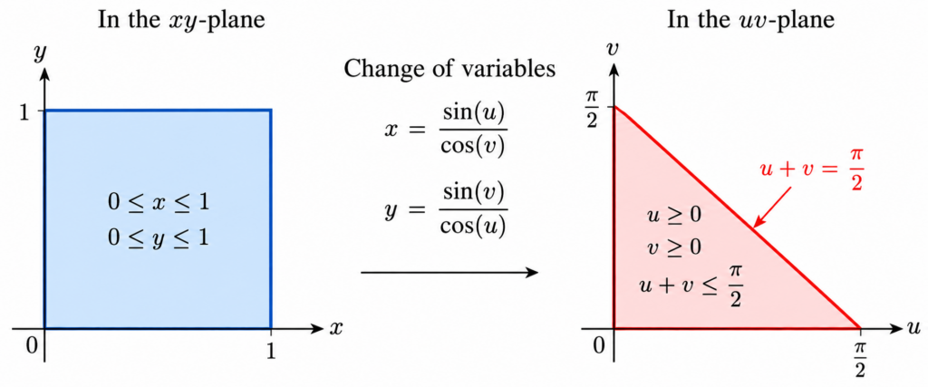
Now comes the surprising part. Introduce new variables u and v by
$x = \frac{\sin (u)}{\cos (v)}, y = \frac{\sin (v)}{\cos (u)} .$
The square
$0 \leq x \leq 1, 0 \leq y \leq 1$
corresponds to the triangular region
$u \geq 0, v \geq 0, u + v \leq \frac{π}{2} .$
To see where the last boundary comes from, notice that
$x \leq 1 \Leftrightarrow \sin (u) \leq \cos (v) \Leftrightarrow u + v \leq \frac{π}{2},$
and the condition on y gives the same inequality.

The Jacobian

We compute
$\frac{\partial x}{\partial u} = \frac{\cos (u)}{\cos (v)}, \frac{\partial x}{\partial v} = \frac{\sin (u) \sin (v)}{{\cos (v)}^{2}} .$
Similarly,
$\frac{\partial y}{\partial u} = \frac{\sin (u) \sin (v)}{{\cos (u)}^{2}}, \frac{\partial y}{\partial v} = \frac{\cos (v)}{\cos (u)} .$
After simplifying the determinant, the Jacobian is
$\frac{\partial (x, y)}{\partial (u, v)} = 1 - x^{2} y^{2} .$
This is exactly the expression that appears in the denominator of our original integral. Therefore,
$\frac{d x d y}{1 - x^{2} y^{2}} = d u d v .$
The complicated-looking integrand has completely disappeared.

The integral becomes an area

Our double integral is now simply
$I = \int_{0}^{\frac{π}{2}} \int_{0}^{\frac{π}{2} - u} d v d u .$
Geometrically, this is the area of a right triangle whose two perpendicular sides both have length
$\frac{π}{2}$
Therefore,
$I = \frac{1}{2} \cdot \frac{π}{2} \cdot \frac{π}{2} = \frac{π^{2}}{8} .$
We have proved that
$1 + \frac{1}{3^{2}} + \frac{1}{5^{2}} + \frac{1}{7^{2}} + \dots = \frac{π^{2}}{8} .$
Recovering the full series

Let
$T = \sum_{n = 1}^{\infty} \frac{1}{n^{2}} .$
Split the series into its odd and even terms. The odd terms have sum
$\frac{π^{2}}{8}$
while the even terms have sum
$\frac{1}{2^{2}} + \frac{1}{4^{2}} + \frac{1}{6^{2}} + \dots = \frac{1}{4} T .$
Consequently,
$T = \frac{π^{2}}{8} + \frac{1}{4} T .$
Thus,
$\frac{3}{4} T = \frac{π^{2}}{8},$
and finally,
$T = \frac{π^{2}}{6} .$
Why this proof is remarkable

We started with an infinite series involving nothing but reciprocals of squares. We then represented part of that series by a double integral over a square. A carefully chosen trigonometric change of variables transformed the square into a triangle and, at the same time, made the integrand disappear.

The infinite series was therefore reduced to the area of a triangle:
$\frac{1}{2} \cdot \frac{π}{2} \cdot \frac{π}{2} = \frac{π^{2}}{8} .$
From there, separating the odd and even terms gives the celebrated result
$\sum_{n = 1} \frac{1}{n^{2}} = \frac{π^{2}}{6} .$
It is a striking example of how an infinite series, a double integral, a trigonometric substitution, and a simple geometric area can all describe the same number.

Another Problem Where Two Dimensions Help

The double-integral proof of the Basel sum illustrates a powerful mathematical idea: sometimes a problem becomes easier when we move to a higher dimension.

One of the most beautiful examples is the Gaussian integral. A one-dimensional integral that resists ordinary antiderivative methods becomes accessible after it is squared and transformed into a two-dimensional integral.

Continue exploring: The Gaussian Integral and Beyond: From e^(-x²) to a Family of Integrals

Long before Euler solved the Basel problem, ancient Greek mathematicians had developed ingenious geometric methods for evaluating infinite sums. In particular, Archimedes used areas of triangles to establish a remarkable infinite series identity. Discover his method in How the Ancient Greeks Summed Infinite Series Without Calculus .

September 28, 2026