Tag: Geometry

  • Marden’s Theorem: How the Derivative of a Cubic Finds an Ellipse

    What can the derivative of a polynomial tell us about geometry? For a cubic polynomial with three complex roots, the answer is surprisingly precise: the derivative locates the two foci of a particular ellipse.

    Let

    p(z) = (z−z1) (z−z2) (z−z3),

    where z1, z2, z3 are three distinct, noncollinear complex numbers.

    Every complex number can be represented as a point in the complex plane. Therefore the three roots of p become three points, and those three points form a triangle.

    Now differentiate. Since p is cubic, p′(z) is quadratic and has two roots, counted with multiplicity. Call them w1 and w2.

    Where are these two critical points located, and what do they have to do with the triangle formed by the original three roots?
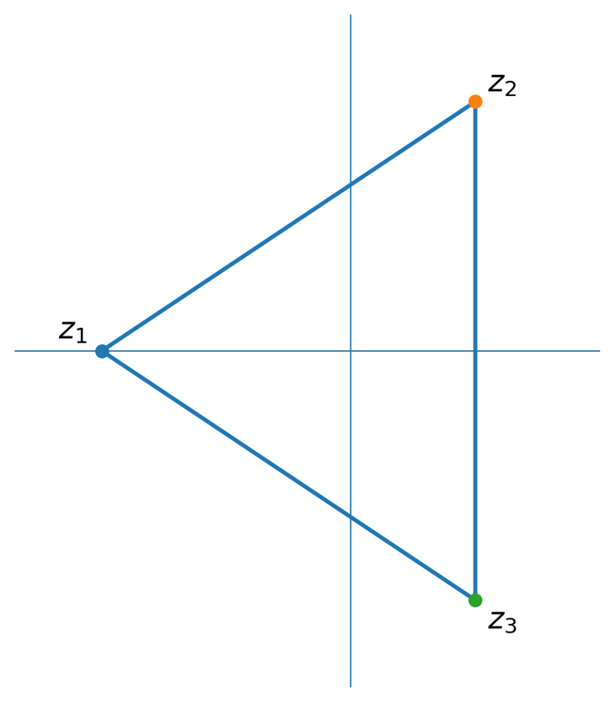
    Three complex roots z1, z2, and z3 plotted as points in the complex plane and joined to form a triangle.
    Figure 1. Three noncollinear roots z₁, z₂, and z₃ of a cubic polynomial determine a triangle in the complex plane.

    What does the derivative know about the triangle?

    There is already a classical theorem that gives us some information. The Gauss–Lucas theorem states that the zeros of the derivative of a polynomial lie in the convex hull of the zeros of the polynomial.

    For our cubic, the convex hull of the three roots is simply the triangle with vertices z1, z2, z3. Therefore the two zeros of p′ must lie inside this triangle.

    That is already an interesting connection between differentiation and geometry. But for a cubic, something much stronger is true.
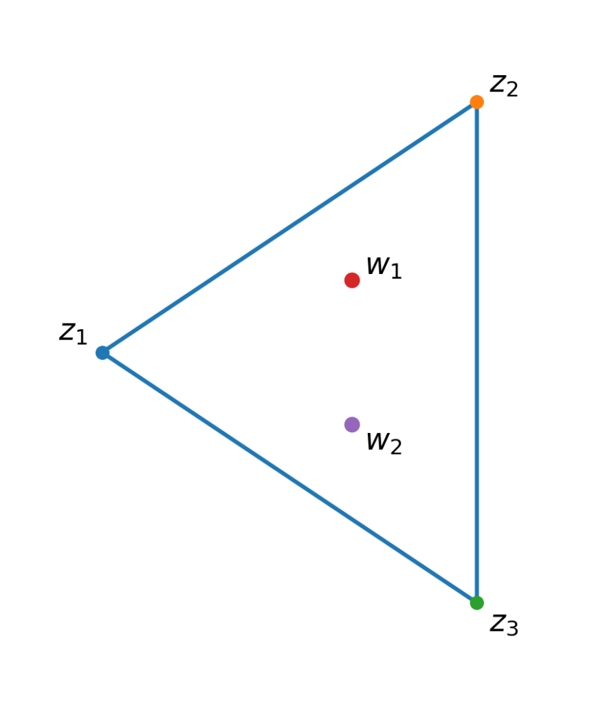
    Triangle formed by three complex roots z1, z2, and z3, with the two derivative zeros w1 and w2 shown inside the triangle.
    Figure 2. By the Gauss–Lucas theorem, the two zeros w₁ and w₂ of the derivative lie inside the triangle determined by the three roots of the cubic.

    Marden’s theorem

    Recall the Steiner inellipse of a triangle: the unique ellipse tangent to the three sides at their midpoints.

    We discussed this ellipse and an area characterization of it in The Steiner Inellipse and a Surprising Area Characterization .

    Marden’s theorem reveals a completely different way in which the same ellipse appears.

    Marden’s Theorem. Let

    p(z) = (z−z1) (z−z2) (z−z3),

    where the three roots are noncollinear. Then the two zeros of p′(z) are exactly the two foci of the Steiner inellipse of the triangle whose vertices are z1, z2, z3.

    This is much stronger than Gauss–Lucas. Gauss–Lucas tells us that the critical points are somewhere inside the triangle. Marden’s theorem identifies their exact geometric meaning.

    The derivative of the cubic has found the foci of an ellipse determined by the roots of the original polynomial.
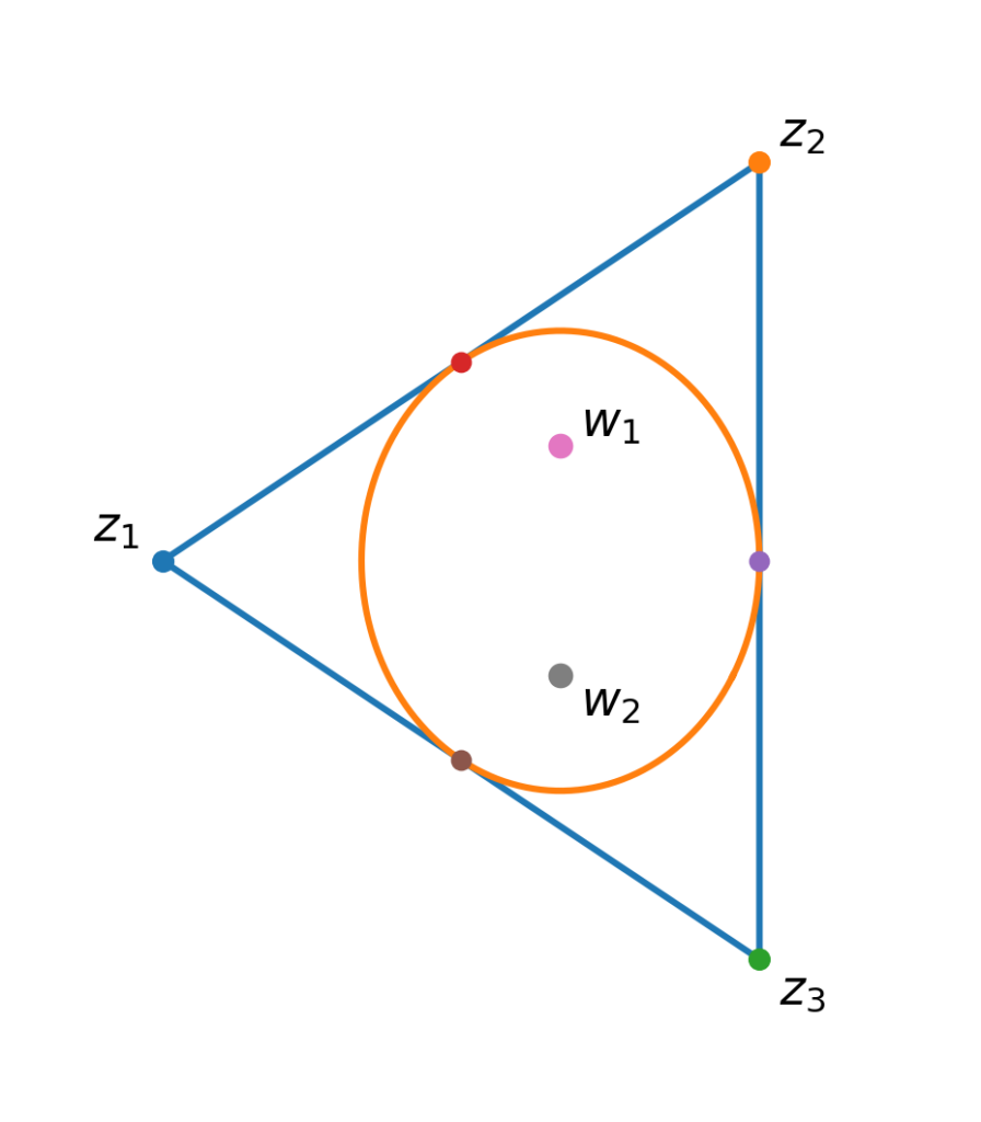
    Triangle formed by three complex roots with its Steiner inellipse tangent at the side midpoints. The two zeros of the derivative are marked at the two foci of the ellipse.
    Figure 3. Marden’s theorem: the two zeros w₁ and w₂ of the derivative are exactly the foci of the Steiner inellipse of the triangle formed by z₁, z₂, and z₃.

    A concrete example

    Let us see the theorem in action. Choose the three roots

    z1=−2, z2=1+2i, z3=1−2i.

    The corresponding cubic is

    p(z) = (z+2) (z−1−2i) (z−1+2i).

    Multiplying the conjugate factors first gives

    (z−1−2i) (z−1+2i) = z2 −2z +5.

    Hence

    p(z) = (z+2) ( z2 −2z +5 ) = z3 +z +10.

    Now differentiate:

    p′(z) = 3z2 +1.

    The critical points satisfy

    3z2 +1 =0,

    so

    z = ± i 3 .

    Marden’s theorem now tells us something geometric that would be very difficult to guess merely by looking at the polynomial:

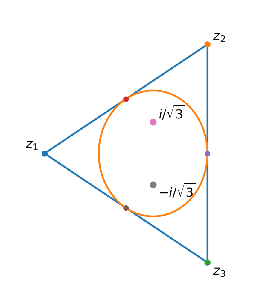
    The two foci of the Steiner inellipse are
    i3 and − i3.
    Triangle with complex roots negative 2, 1 plus 2i, and 1 minus 2i, together with its Steiner inellipse. The two foci are located at i over square root of 3 and negative i over square root of 3.
    Figure 4. For p(z) = z³ + z + 10, the roots form the displayed triangle, while the zeros ±i/√3 of p′(z) are exactly the foci of its Steiner inellipse.

    Why is this so surprising?

    The derivative is usually introduced as an analytic object: it measures instantaneous rate of change, gives the slope of a tangent line, and locates critical points.

    Here it is doing something that looks completely different.

    Start with three complex numbers. Use them as the roots of a cubic. Differentiate the polynomial. Solve one quadratic equation. The two answers are not merely points somewhere inside the triangle—they are the two foci of a distinguished ellipse.

    In symbols, the chain of ideas is

    three roots → triangle → differentiate → two critical points → two foci.

    The same Steiner inellipse therefore admits two very different descriptions.

    In our earlier article, it appeared from an area condition: a point lies on the ellipse precisely when three corner triangles have total area equal to half the area of the original triangle.

    Here the ellipse appears from differentiation: its two foci are the zeros of the derivative of the cubic whose roots are the vertices of the triangle.

    This is a beautiful example of a recurring theme in mathematics: algebra, calculus, and geometry can encode the same object in completely different ways.

    References and further reading

    1. D. Kalman, “An Elementary Proof of Marden’s Theorem” , The American Mathematical Monthly, Vol. 115, No. 4 (2008), pp. 330–338.
    2. A. Eydelzon, “On a New Property of the Steiner Inellipse” , The American Mathematical Monthly, Vol. 127, No. 10 (2020), pp. 933–935.
  • Can a Curve Fill a Square? The Mathematics of Space-Filling Curves

    Can a Curve Fill a Square?

    A curve is one-dimensional. A square is two-dimensional. So it seems impossible that a single continuous curve could pass through every point of a square.

    Surprisingly, it can.

    There exists a continuous function

    H : [0,1] → [0,1] × [0,1]

    whose image is the entire unit square. In other words, as the parameter moves continuously from 0 to 1, the point H(t) eventually reaches every point of the square.

    Such a curve is called a space-filling curve.

    The Hilbert Curve

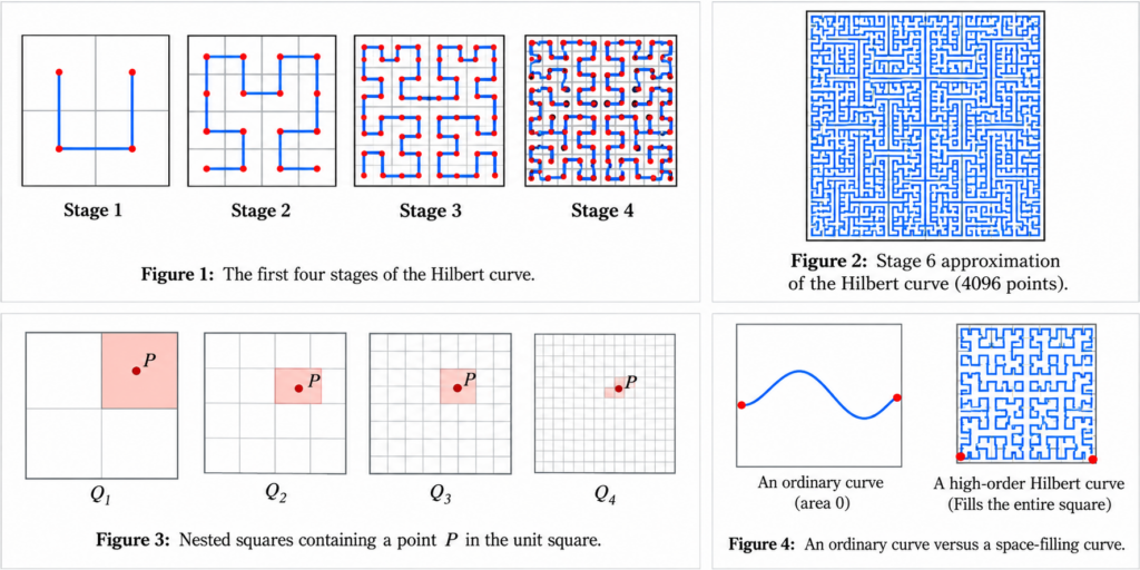
    One of the most beautiful examples is the Hilbert curve. Instead of trying to draw the final curve immediately, we construct a sequence of increasingly complicated polygonal curves.

    Start with a square. Divide it into four equal smaller squares and connect their centers in an order that forms a U-shaped path.

    This is the first approximation.

    For the second approximation, divide each of the four squares into four smaller squares. We now have

    42 = 16

    small squares. Inside each group of four, place a suitably rotated or reflected copy of the previous pattern and connect the pieces.

    Repeat the process again and again.

    At stage n, the square has been divided into

    4n

    small squares, each having side length

    2 −n .

    The Squares Become Tiny

    The important feature of the construction is not merely that the number of squares increases. Their size simultaneously decreases to zero.

    A small square at stage n has side length

    12n,

    so its diameter is

    2 2n .

    Therefore,

    2 2n → 0 as n → ∞.

    The construction is examining the square on smaller and smaller scales.

    Why Does the Limit Fill the Square?

    Take any point P in the unit square.

    At the first stage, P belongs to at least one of the four small squares. Call one such square Q1.

    At the second stage, choose one of the smaller squares containing P and call it Q2. Continue in this way.

    We obtain nested squares

    Q1 ⊇ Q2 ⊇ Q3 ⊇ ⋯

    containing P, while

    diam ( Qn ) → 0.

    Since the squares shrink to a point, their intersection is precisely

    ⋂ n=1 ∞ Qn = {P}.

    The Hilbert construction assigns corresponding nested parameter intervals

    I1 ⊇ I2 ⊇ I3 ⊇ ⋯

    whose lengths also tend to zero. Their intersection therefore determines a parameter value t. For this value,

    H (t) = P.

    But P was an arbitrary point of the square. Thus the limiting curve reaches every point of the square.

    A Curve Whose Image Has Area 1

    This produces a remarkable conclusion.

    The domain of the Hilbert curve is the interval [0,1], but its image is

    H ( [0,1] ) = [0,1] × [0,1].

    Consequently, the image of this continuous curve has area

    1.

    This is very different from an ordinary smooth curve, whose area in the plane is zero.

    What Happens to the Length?

    The polygonal approximations also reveal something interesting.

    At stage n, the curve visits 4n small squares. The characteristic distance between neighboring points is of order

    2 −n .

    Therefore the total length is of order

    4n · 2 −n = 2n.

    As n→∞, this quantity tends to infinity.

    2n → ∞.

    Thus the approximations stay inside a square of area 1, but their lengths grow without bound.

    Does This Mean an Interval and a Square Are the Same?

    No.

    The Hilbert curve is continuous and onto, but it is not one-to-one. Different parameter values can correspond to the same point of the square.

    This distinction is essential. There is no continuous one-to-one correspondence with a continuous inverse between an interval and a square.

    The space-filling curve does something subtler: it continuously folds an interval over itself infinitely many times until its image covers the entire square.

    A Dimensional Clue

    There is another way to see why the numbers in the construction fit together so naturally.

    When lengths are reduced by a factor of 2, the number of pieces increases by a factor of 4:

    4 = 22.

    If we informally ask for a dimension d satisfying

    4 = 2d,

    then

    d = log4 log2 = 2.

    This scaling behavior gives a hint of how a construction beginning with a one-dimensional parameter can produce an image that occupies a two-dimensional region.

    Why Space-Filling Curves Are Useful

    Space-filling curves are not only mathematical curiosities. Hilbert-type orderings are useful whenever multidimensional data must be arranged in a one-dimensional sequence.

    The Hilbert ordering has an important locality property: points that are close along the curve tend to remain relatively close in space. This idea appears in spatial indexing, image processing, databases, and algorithms for organizing multidimensional data.

    A construction that originally seemed almost paradoxical therefore connects pure mathematics with practical computation.

    The Main Idea

    The Hilbert curve demonstrates how misleading our finite-dimensional intuition can be when a limiting process is repeated infinitely many times.

    Every finite approximation is just an ordinary polygonal curve. None of these approximations fills the square.

    But the subdivisions become arbitrarily small, and in the limit every point of the square is reached.

    A continuous image of a one-dimensional interval can therefore fill an entire two-dimensional square.


    Continue exploring: Another surprising example of how strange continuous functions can be: Can a Function Be Continuous Everywhere but Differentiable Nowhere?

    Not all interesting curves are as unusual as space-filling curves. Some are designed to create smooth, controllable shapes using only a few points. Discover how this works in Bézier Curves: How Four Points Create Beautiful Shapes .