Drag Force – Elite Math Program

One of the most beautiful problems in calculus asks:

What path allows an object, starting from rest, to travel between two points under gravity in the least possible time?

The shortest path is a straight line. But the fastest path is not. In the classical brachistochrone problem, the answer is a cycloid.

But there is an assumption hidden inside this famous result: there is no resistance.

What happens if the object moves through a fluid? Is the fastest path in water, oil, or another viscous medium still a cycloid?

The answer is no longer universal. Once resistance is present, the optimal path depends on the law of motion itself.

1. The Classical Brachistochrone

Suppose an object starts from rest and moves under gravity without friction. Let y measure vertical distance downward from the starting point.

Conservation of energy gives

\frac{1}{2} m v^{2} = m g y .

Therefore

v = \sqrt{2 g y} .

If s denotes distance measured along the curve, then speed is

v = \frac{d s}{d t} .

Therefore

d t = \frac{d s}{v} .

The total travel time is consequently

T = \int \frac{d s}{\sqrt{2 g y}} .

For a curve written as y = y(x),

d s = \sqrt{1 + {\frac{d y}{d x}}^{2}} d x .

Thus

T = \int \frac{\sqrt{1 + {\frac{d y}{d x}}^{2}}}{\sqrt{2 g y}} d x .

Minimizing this integral leads to the cycloid.

2. The Exact Cycloid

With y positive downward, the cycloid can be parametrized as

x (θ) = a (θ - \sin (θ)),

y (θ) = a (1 - \cos (θ)) .

The constants are determined by the endpoint.

The cycloid illustrates the central idea behind the brachistochrone. The curve initially descends very steeply. Although this makes the path longer than a straight line, the object gains speed quickly and then uses that speed during the remainder of the trip.

3. What Changes When There Is Resistance?

The classical derivation relies on conservation of mechanical energy. With drag, mechanical energy is continually dissipated.

Consequently, the speed can no longer be determined from height alone. Two objects arriving at the same height along two different paths may have different speeds because they have experienced different histories of drag.

This destroys the simple relation

v = \sqrt{2 g y} .

Now the path and the velocity must be determined together.

4. Linear Drag

A particularly useful mathematical model assumes that the drag force is proportional to speed:

F_{D} = b v .

For a small sphere in the Stokes regime,

b = 6 π μ R,

where μ is the dynamic viscosity and R is the radius of the sphere.

Let s denote arc length along the unknown path. Since

v = \frac{d s}{d t},

the tangential equation of motion is

m \frac{d v}{d t} = m g \frac{d y}{d s} - b v .

Using

\frac{d v}{d t} = \frac{d v}{d s} \frac{d s}{d t} = v \frac{d v}{d s}

we obtain

m v \frac{d v}{d s} = m g \frac{d y}{d s} - b v .

5. What Are We Minimizing?

The quantity we want to minimize is the total travel time. By definition,

v = \frac{d s}{d t} .

Solving for the small amount of time required to travel the distance ds gives

d t = \frac{d s}{v} .

Therefore, for a path of total length S,

T = \int_{0}^{S} \frac{d s}{v} .

In words,

time = distance / speed.

The important difference from the classical brachistochrone is that, in the presence of drag, the speed v is not determined by height alone. It depends on how the object arrived at its current position.

Thus the viscous brachistochrone problem is to find a path and its corresponding velocity that satisfy the equation of motion while making the total travel time as small as possible.

6. Buoyancy

If the object is immersed in a fluid, buoyancy can also be included. For a body of density ρ_s in a fluid of density ρ_f, the effective downward acceleration is

g_{eff} = g (1 - \frac{ρ_{f}}{ρ_{s}}) .

In the equation of motion, g can then be replaced by g_eff.

7. Water Does Not Automatically Mean Linear Drag

There is an important physical qualification. Stokes’ linear drag law applies only in an appropriate low-Reynolds-number regime.

The Reynolds number is

Re = \frac{ρ v L}{μ} .

At higher Reynolds numbers, a quadratic drag model is often more appropriate:

F_{D} = \frac{1}{2} ρ_{f} C_{D} A v^{2} .

k = \frac{1}{2} ρ_{f} C_{D} A,

then the corresponding tangential equation is

m v \frac{d v}{d s} = m g \frac{d y}{d s} - k v^{2} .

So there is no single mathematical object called the underwater brachistochrone. The answer depends on the object, the fluid, and the appropriate drag law.

8. A Numerical Example

Let us compare two minimum-time paths having the same endpoints:

(0, 0) and (3, 2) .

As before, y is measured downward.

Case A: No Drag

For the classical cycloid,

x = a (θ - \sin (θ)),

y = a (1 - \cos (θ)) .

The endpoint conditions give approximately

θ_{f} \approx 3.068777, a \approx 1.001327 .

Selected points on the exact cycloid are:

θ	x	y
0.0000	0.0000	0.0000
0.3069	0.0048	0.0468
0.6138	0.0379	0.1828
0.9206	0.1248	0.3952
1.2275	0.2862	0.6643
1.5344	0.5358	0.9649
1.8413	0.8788	1.2689
2.1481	1.3120	1.5479
2.4550	1.8235	1.7758
2.7619	2.3944	1.9313
3.0688	3.0000	2.0000

Case B: Linear Drag

Now keep the same endpoints but introduce linear resistance with

\frac{b}{m} = 1.0 s^{- 1},

and take

g = 9.81 \frac{m}{s^{2}} .

This is a mathematical linear-drag example. We do not label it “water” or “oil,” because identifying a real fluid requires checking which drag law is physically appropriate.

The unknown curve can be approximated numerically by short segments. For each candidate path, the equation of motion is integrated along the path, the travel time is computed, and the intermediate heights are varied to reduce that time.

Selected points from the numerical minimum-time path are:

x	y
0.000	0.000
0.300	0.581
0.600	0.913
0.900	1.181
1.200	1.406
1.500	1.595
1.800	1.749
2.100	1.870
2.400	1.955
2.700	1.997
3.000	2.000

9. Something Unexpected Happens

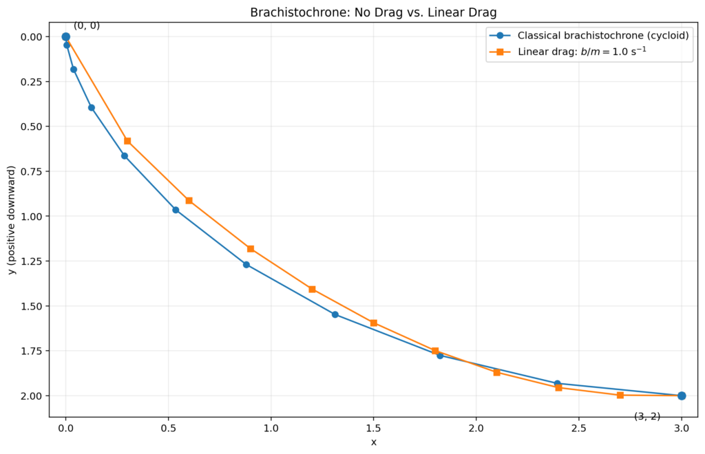
It is tempting to imagine that adding resistance simply moves the entire brachistochrone to one side of the classical cycloid.

The numerical example shows that this is not what happens.

For comparison, evaluating the classical cycloid at the same horizontal positions gives approximately:

x	Linear-drag y	Cycloid y
0.0	0.000	0.000
0.3	0.581	0.684
0.6	0.913	1.029
0.9	1.181	1.285
1.2	1.406	1.484
1.5	1.595	1.643
1.8	1.749	1.767
2.1	1.870	1.863
2.4	1.955	1.932
2.7	1.997	1.978
3.0	2.000	2.000

At x = 1.8, the linear-drag path has y approximately 1.749, while the cycloid has y approximately 1.767.

But at x = 2.1, the linear-drag path has y approximately 1.870, while the cycloid has y approximately 1.863.

Therefore the two curves cross somewhere between these positions.

This is a useful warning against relying only on intuition. Resistance does not merely shift the classical cycloid uniformly upward or downward. It changes the optimization problem itself and can change the shape in a more subtle way.

10. Why Does Drag Change the Answer?

In the frictionless problem, speed gained early is retained. This makes a steep initial descent extremely valuable.

With drag, there is a competing effect. Descending early still produces speed, but resistance continually removes energy. Speed acquired early is therefore not as valuable as it is in the frictionless problem.

The optimal curve must balance:

gaining speed quickly by descending,
the extra distance caused by that descent, and
the continual loss of energy to resistance.

That competition produces a different minimum-time path.

11. There Is No Single “Brachistochrone in Water”

This is perhaps the most important physical lesson.

Changing the medium can change the viscosity, density, buoyancy, Reynolds number, drag coefficient, and even the mathematical form of the drag law. Changing the size or shape of the moving object can do the same.

Therefore asking

“What is the brachistochrone in water?”

does not completely specify the problem.

A more precise question is:

For this object, in this fluid, under this drag law, what path minimizes the travel time?

12. The Bigger Lesson

The classical brachistochrone is famous because the answer is unexpectedly beautiful: a cycloid.

But there is an even broader lesson hiding behind it.

The fastest path is not determined by geometry alone. It depends on the law of motion.

With no resistance, the answer is a cycloid. With viscous resistance, the speed remembers the history of the path, and the optimization problem changes. For other drag laws, it changes again.

So perhaps the more interesting question is not

“What is the fastest curve?”

but rather

“What physical laws make a particular curve the fastest?”

Classical cycloid and numerical linear-drag brachistochrone from (0, 0) to (3, 2), showing the two optimal paths crossing.

Another example where the mathematics of motion produces a surprising result is my related-rates problem about a sliding ladder: is it safer to slide or jump?

Tag: Drag Force

Is the Brachistochrone Still a Cycloid Underwater?