Cone Fitting – Elite Math Program

Several years ago, I was given an applied mathematics problem that sounded simple at first:

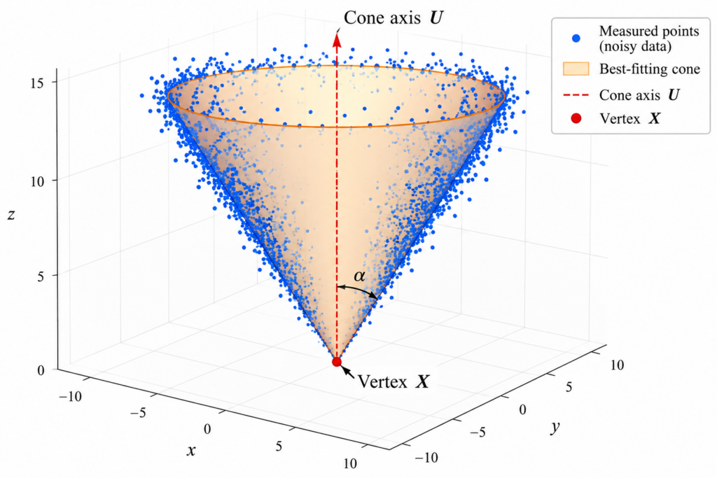
Given thousands of measured points in three-dimensional space, find the cone that best fits them.

But there was an additional requirement that changed the problem completely. The calculation had to be fast enough to be used in real time.

It is one thing to describe an optimization problem mathematically. It is another thing to solve it repeatedly, quickly, and reliably while a real system is operating.

The solution came from combining elementary geometry with nonlinear least squares and the Gauss–Newton method.

The Geometric Problem

Suppose a collection of measured points

P_{1}, P_{2}, \dots, P_{m}

lies close to the surface of an unknown right circular cone.

We want to determine three things:

the vertex of the cone, the direction of its axis, and its opening angle.

Let

X = (x_{1}, x_{2}, x_{3})

be the vertex, let $U$ point along the axis, and let $α$ be the half-angle of the cone.

If $P$ lies exactly on the cone, then the vector

P - X

makes angle $α$ with the cone axis.

The dot-product formula for the angle between two vectors therefore gives

{({(P - X)}^{T} U)}^{2} = {‖ P - X ‖}^{2} {‖ U ‖}^{2} {cos α}^{2} .

This one equation contains the geometry of the cone.

Turning Geometry into an Error

Measured data will not lie exactly on a perfect cone. There will be noise, measurement error, and small deviations from the ideal surface.

So instead of asking whether a point satisfies the cone equation exactly, we measure how far it is from satisfying the equation.

Define the residual

R (P) = {‖ P - X ‖}^{2} {cos α}^{2} - \frac{{({(P - X)}^{T} U)}^{2}}{{‖ U ‖}^{2}} .

For a point exactly on the cone,

R (P) = 0 .

For a measured point near the cone, the residual will generally be nonzero.

Why Use This Residual?

There is an important practical point here.

One could try to calculate the exact shortest geometric distance from every measured point to the cone. But when thousands of points must be processed repeatedly in real time, the computational form of the problem matters.

The residual above is obtained directly from the cone equation. It can be evaluated using additions, multiplications, dot products, and a few simple functions.

This was exactly what was needed for the application: a mathematical description that could be differentiated explicitly and evaluated rapidly.

Six Unknown Parameters

The direction of the axis does not depend on the length of $U$ . Multiplying the axis vector by a nonzero constant gives the same axis.

Assuming the axis is not parallel to the $(x_{1}, x_{2})$ plane, we can therefore write

U = (u_{1}, u_{2}, 1) .

The entire cone is then described by only six unknown numbers:

S = {(x_{1}, x_{2}, x_{3}, u_{1}, u_{2}, α)}^{T} .

Three numbers locate the vertex, two determine the axis direction, and one determines the cone angle.

From One Point to Thousands of Points

Suppose there are $m$ measured points.

For each point $P_{j}$ , compute a residual $R_{j}$ .

We then look for the cone that minimizes the total squared residual:

f (S) = \frac{1}{2} \sum_{j = 1}^{m} R_{j}^{2} .

This is a nonlinear least-squares problem.

Why Not Just Solve the Equations?

If the measurements were perfect, six carefully chosen points might appear to be enough to determine six unknown parameters.

Real data do not work that way.

Measurements contain noise, and a small collection of points may give a poor estimate. Instead, we can use hundreds or thousands of points simultaneously and find the cone that best fits all of them.

But now the equations are nonlinear. There is no simple matrix formula that immediately gives the answer.

This is where Gauss–Newton enters the story.

The Jacobian

Put all the residuals into one vector:

E = {(R_{1}, R_{2}, \dots, R_{m})}^{T} .

Then

f = \frac{1}{2} {‖ E ‖}^{2} .

The Jacobian $J$ contains the derivatives of every residual with respect to the six cone parameters.

Its $j$ -th row is

J_{j} = (\frac{\partial R_{j}}{\partial x_{1}}, \frac{\partial R_{j}}{\partial x_{2}}, \frac{\partial R_{j}}{\partial x_{3}}, \frac{\partial R_{j}}{\partial u_{1}}, \frac{\partial R_{j}}{\partial u_{2}}, \frac{\partial R_{j}}{\partial α}) .

In the actual implementation, these derivatives were derived analytically rather than estimated numerically.

That requires more work at the beginning, but once the formulas are known, they can be evaluated very efficiently.

The Key Gauss–Newton Approximation

The gradient of the least-squares objective has a particularly simple form:

\nabla f = J^{T} E .

The exact Hessian is

\nabla^{2} f = J^{T} J + \sum_{j = 1}^{m} R_{j} \nabla^{2} R_{j} .

Computing the second term repeatedly is considerably more expensive.

Gauss–Newton makes the approximation

\nabla^{2} f \approx J^{T} J .

This approximation becomes especially natural when the fit is already good, because the residuals $R_{j}$ are then small.

That observation was crucial for a real-time implementation. Instead of constructing the complete second derivative at every iteration, we can work primarily with the Jacobian.

One Iteration

At the current estimate $S_{k}$ , the Gauss–Newton direction $G_{k}$ is obtained by solving

{J_{k}}^{T} J_{k} G_{k} = - {J_{k}}^{T} E_{k} .

Then update the six cone parameters:

S_{k + 1} = S_{k} + a_{k} G_{k} .

Here $0 < a_{k} \leq 1$ is the step length.

Why Use a Line Search?

Taking the full Gauss–Newton step is not always a good idea when the current estimate is still far from the solution.

The implementation therefore reduces the step when necessary until the objective function decreases sufficiently.

In mathematical form, choose the step length so that

f (S_{k} + a_{k} G_{k}) \leq f (S_{k}) + ρ a_{k} {\nabla f_{k}}^{T} G_{k} .

The purpose is simple: do not accept an iteration that moves too aggressively in a direction that fails to improve the fit sufficiently.

The Real-Time Idea

At first glance this may still look like a large calculation. There may be thousands of measured points.

But notice something important.

No matter how many data points we have, there are still only six unknown cone parameters.

The Jacobian may have thousands of rows, but only six columns. The matrix

J^{T} J

is therefore only

6 \times 6 .

Similarly,

J^{T} E

has only six components.

So the data set can be large while the system that must be solved at each Gauss–Newton iteration remains very small.

This is exactly the type of structure one wants to exploit in a real-time numerical algorithm.

Did It Work?

Yes.

This was not an exercise invented to demonstrate Gauss–Newton. I developed the method because the cone-fitting calculation was needed in a real application, and it had to operate in real time.

The implementation worked extremely well.

That experience taught me an important lesson about applied mathematics: the best mathematical formulation is not necessarily the one that looks most sophisticated on paper.

Sometimes the decisive question is:

Can we formulate the problem so that the computer can solve it quickly enough to be useful?

Why the Approximation Works

There is another nice feature of Gauss–Newton.

Recall that the exact Hessian is

\nabla^{2} f = J^{T} J + \sum_{j = 1}^{m} R_{j} \nabla^{2} R_{j} .

As the estimated cone approaches the data, the residuals become small. Consequently, the second term becomes less important and

\nabla^{2} f \approx J^{T} J .

So as the algorithm approaches a good fit, the inexpensive approximation becomes increasingly appropriate.

A Final Check

Although computing the full Hessian at every iteration is expensive, it can still be useful after the optimization has finished.

At the final solution we can evaluate

\nabla^{2} f = J^{T} J + \sum_{j = 1}^{m} R_{j} \nabla^{2} R_{j} .

If its eigenvalues are positive, the Hessian is positive definite and the computed stationary point is a local minimum.

In other words, we use the inexpensive approximation while speed matters, and we can use the more expensive calculation afterward as a check.

The Larger Lesson

The mathematics of this problem can be summarized in one chain:

3D measurements → cone geometry → residuals → least squares → Jacobian → Gauss–Newton → real-time fit.

The cone itself is elementary geometry. Least squares is a classical idea. The derivatives require calculus. Gauss–Newton comes from numerical optimization.

None of these ingredients alone solves the practical problem.

The solution comes from putting them together in a form that a computer can evaluate rapidly.

That is one of the most satisfying aspects of applied mathematics: sometimes a few familiar mathematical ideas, combined in the right way, turn a difficult real-world computation into something that works almost like magic.

A Closely Related Fitting Problem

Fitting a cone to a large cloud of measured points is one example of a broader problem: how can we recover a geometric surface accurately when the computation has to be fast enough for real-time use?

A closely related problem replaces the cone by a cylinder. The geometry changes, but the same practical challenge remains: turn thousands of measurements into a reliable geometric fit without an expensive general-purpose optimization.

Continue exploring: How Do You Fit a Cylinder to Thousands of Points in Real Time?

Tag: Cone Fitting

How Do You Fit a Cone to Thousands of Points in Real Time?