Tag: Carrying Capacity

“`html

A remarkably simple differential equation appears in many different places in the real world. We will begin with population growth. The first model we try will have a serious problem: it predicts unlimited growth. Fixing that problem will lead us to the logistic equation.

Then, surprisingly, we will return to our original equation and discover that it was not a bad equation at all. The same equation describes continuous compound interest, radioactive decay, and many other processes.

1. The Simplest Population Model

Let $P\left(t\right)$ denote a population at time $t$.

One of the simplest assumptions we can make is this: the rate at which the population grows is proportional to the population itself.

$$\frac{dP}{dt}=kP,P\left(0\right)=P_0.$$

Here $k>0$ is a constant. The idea seems reasonable. If there are twice as many individuals, we might expect approximately twice as many births. A larger population therefore grows faster.

The equation is separable:

$$\frac{dP}{P}=kdt.$$

Integrating gives

$$\ln P=kt+C,$$

and therefore

$$P\left(t\right)=P_0{e}^{kt}.$$

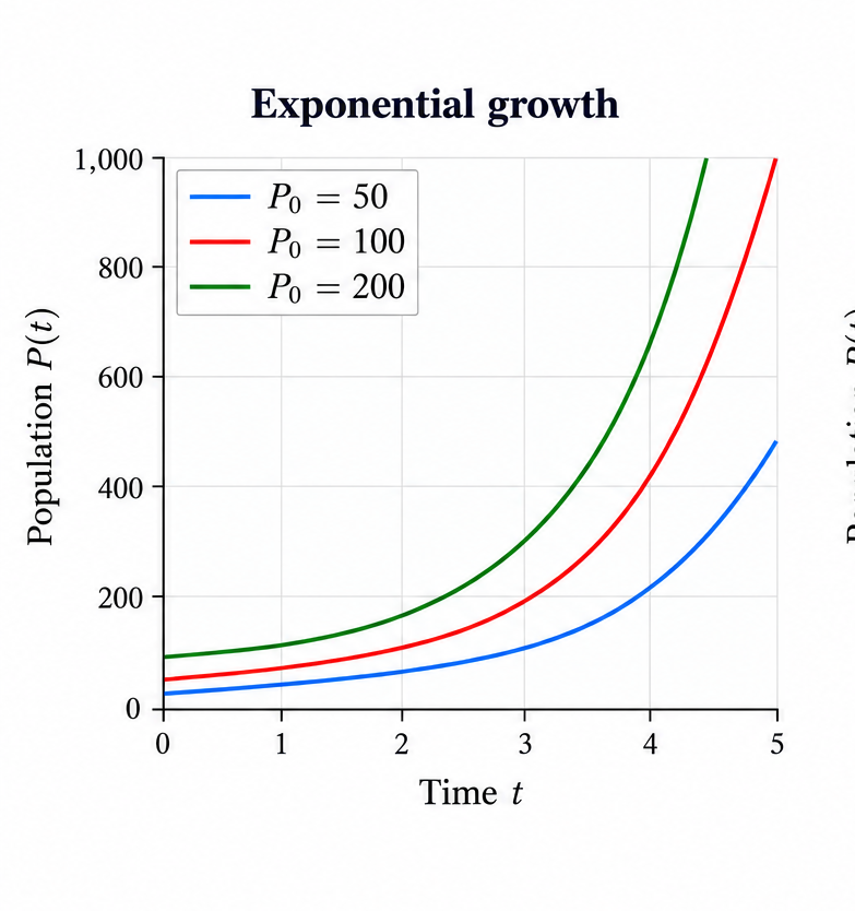
This is exponential growth.

There is an immediate problem. If $k>0$, then

$$P\left(t\right)\to \infty \text{as}t\to \infty .$$

According to this model, the population eventually becomes arbitrarily large. That cannot continue indefinitely in the real world. Food, water, space, and other resources are limited.

So our first population model is useful for describing growth over some periods, but it cannot be the whole story.

“`

“`html

2. Introducing a Carrying Capacity

Suppose the environment can sustainably support a maximum population $K$. This number is called the carrying capacity.

We modify our original equation to

$$\frac{dP}{dt}=kP(1-\frac{P}{K})$$

This is the logistic equation.

The new factor

$$(1-\frac{P}{K})$$

is what changes everything. When the population is small compared with $K$, this factor is close to 1, so the population behaves approximately like ordinary exponential growth. As the population becomes larger, the factor becomes smaller and the growth slows down.

We Can Predict the Solutions Without Solving the Equation

This is one of the most useful ideas in differential equations: we do not always need an explicit formula to understand what the solutions will do.

First suppose

$$0<P<K.$$

Then

$$(1-\frac{P}{K})>0,$$

and consequently

$$\frac{dP}{dt}>0.$$

So the population increases.

Now suppose $P=K$. Then

$$(1-\frac{P}{K})=0,$$

so

$$\frac{dP}{dt}=0.$$

The population remains constant at the carrying capacity.

Finally, if $P>K$, then

$$(1-\frac{P}{K})<0,$$

and therefore

$$\frac{dP}{dt}<0.$$

The population decreases toward the carrying capacity.

Where Is the Population Growing Fastest?

The growth rate is

$$kP(1-\frac{P}{K}).$$

As a function of $P$, this is a downward-opening quadratic:

$$kP-\frac{k{P}^2}{K}.$$

Its maximum occurs at

$$P=\frac{K}{2}.$$

This tells us something important about the shape of the population curve.

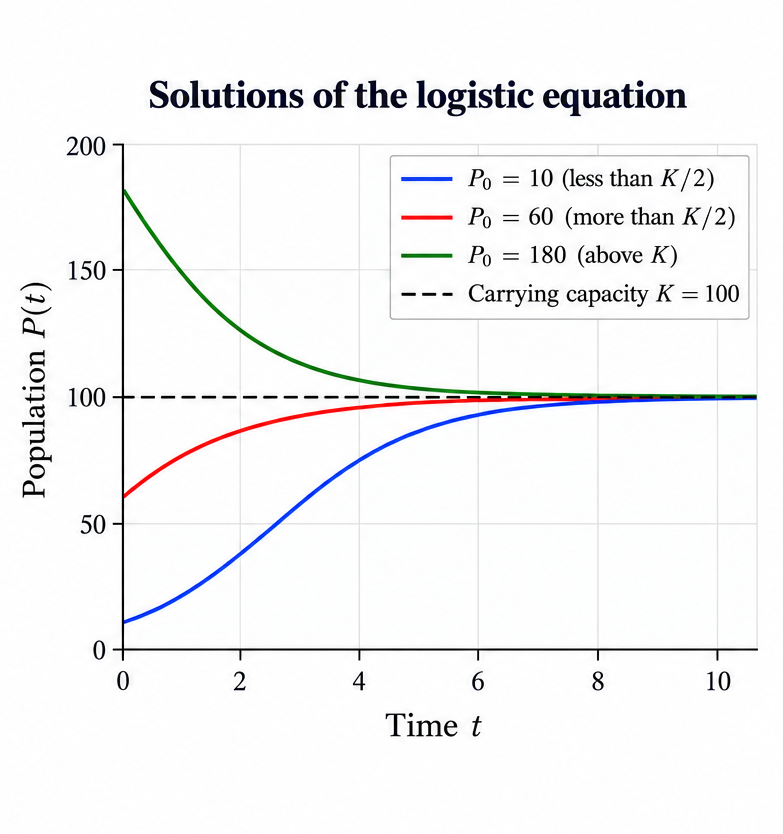
If $P_0<\frac{K}{2}$, the population initially grows faster and faster. When it reaches $P=\frac{K}{2}$, its growth rate is greatest. After that, the population continues to increase, but more and more slowly as it approaches $K$. This produces the familiar S-shaped logistic curve.

If $\frac{K}{2}<P_0<K$, the population begins above the point of fastest growth. It still increases toward $K$, but it slows down from the beginning.

Finally, if $P_0>K$, the population decreases toward $K$.

Thus, before solving the logistic equation, we can already predict the three different types of solution curves shown in the next figure.

“`

“`html id=”p87fcf”

3. Now Let Us Solve the Logistic Equation

We now return to the logistic equation

$$\frac{dP}{dt}=kP(1-\frac{P}{K}),P(0)=P_0.$$

We have already learned a great deal about its solutions without solving it. Now let us find the actual formula.

First separate the variables:

$$\frac{dP}{P(1-\frac{P}{K})}=kdt.$$

Since

$$\frac{1}{P(1-\frac{P}{K})}=\frac{1}{P}+\frac{1}{K-P},$$

we can integrate:

$$\int (\frac{1}{P}+\frac{1}{K-P})dP=\int kdt.$$

This gives

$$\ln P-\ln (K-P)=kt+C.$$

Combining the logarithms,

$$\ln \left(\frac{P}{K-P}\right)=kt+C.$$

Exponentiating both sides gives

$$\frac{P}{K-P}=C{e}^{kt}.$$

Using the initial condition $P(0)=P_0$, we obtain

$$C=\frac{P_0}{K-P_0}.$$

After solving for $P$, we obtain the logistic growth formula:

$$P(t)=\frac{K}{1+\frac{K-P_0}{P_0}{e}^{-kt}}.$$

Now the formula confirms what we predicted from the differential equation. For positive initial populations, the population approaches the carrying capacity:

$$P(t)\to K\text{as}t\to \infty .$$

So the carrying capacity is not merely a number inserted into the model. It becomes the long-term population predicted by the model.

4. Was Our Original Equation Really So Bad?

We rejected the equation

$$\frac{dy}{dt}=ky$$

as a model of population growth over an unlimited period of time. But the equation itself is one of the most important differential equations in mathematics.

The initial-value problem

$$\frac{dy}{dt}=ky,y(0)=y_0$$

has the solution

$$y(t)=y_0{e}^{kt}.$$

What changes from one application to another is the meaning of $y$ and the sign and meaning of the proportionality constant.

5. Continuous Compound Interest

Suppose an amount of money $A(t)$ earns interest continuously at an annual rate $r$. The rate at which the account balance changes is proportional to the amount currently in the account:

$$\frac{dA}{dt}=rA,A(0)=A_0.$$

Therefore,

$$A(t)=A_0{e}^{rt}.$$

The same equation that produced exponential population growth now describes the growth of money.

6. Radioactive Decay

Now consider a radioactive substance. The more radioactive nuclei that are present, the more nuclei are available to decay. Thus, the magnitude of the decay rate is proportional to the amount currently present.

This time the quantity is decreasing, so we write

$$\frac{dN}{dt}=-\lambda N,N(0)=N_0,$$

where $\lambda >0$ is the decay constant.

The solution is

$$N(t)=N_0{e}^{-\lambda t}.$$

7. One Equation, Many Processes

We began with perhaps the simplest population model imaginable: the rate of change of a population is proportional to the population itself.

As a long-term population model, it failed. Unlimited exponential population growth is impossible in an environment with limited resources.

Introducing a carrying capacity led naturally to the logistic equation. Even more importantly, we were able to predict the behavior of its solutions before solving the equation.

But our original equation was far from useless. The same basic mathematical law appears in continuous compound interest and radioactive decay.

The common idea is simple:

The rate of change of a quantity is proportional to the amount of that quantity currently present.

Population, money, and radioactive atoms seem like completely different things. Mathematically, however, they can obey the same law.

That is one of the remarkable features of differential equations: the same mathematical equation can describe very different processes in the real world.

---

Related: See another example where a simple mathematical model produces a surprising—and ultimately unrealistic—prediction: A Sliding Ladder: Is It Better to Slide or Jump? .