Tag: calculus

How the Ancient Greeks Summed Infinite Series Without Calculus
Can infinitely many pieces have a finite total area? The Greeks approached this question through geometric exhaustion. Archimedes proved that a parabolic segment has four-thirds the area of its largest inscribed triangle. Here we explain the geometry with modern notation, clearly distinguishing ancient arguments from modern illustrations.

1. Zeno and infinitely many steps

Travel half a unit, then a quarter, then an eighth, and so on. The infinite subdivision raises Zeno’s famous question: can infinitely many stages have a finite total?
12+14+18+⋯=1
Figure 1. Zeno’s successive halfway distances. This is a modern diagram of the ancient philosophical problem.

After n steps the distance left is 1/2ⁿ. It tends to zero, although no finite step reaches the endpoint.

2. A square proves a geometric series

Partition a unit square into vertical strips of widths 1/2, 1/4, 1/8, … . The strip areas have exactly these values.

Figure 2. Successive strips fill the unit square in the limit. Each new strip is half the remaining width.
Sn=1−12n
Since the unfilled strip has area 1/2ⁿ, its area approaches zero. The same argument gives the general geometric sum when 0 < q < 1:
1+q+q2+⋯=11−q
The colored-square construction and modern series notation are teaching devices, not a reconstruction of a particular surviving ancient proof.

3. Archimedes’ quadrature of the parabola

Consider the region between y = 1 − x² and the chord from (−1,0) to (1,0). Its largest inscribed triangle has vertices (−1,0), (0,1), (1,0), and area T = 1.

Figure 3. The blue triangle has area T. The orange pair totals T/4, and the green group totals T/16. Later generations continue the same pattern.

Why does every generation shrink by a factor of four?

The next triangle on the left has vertices (−1,0), (0,1), and (−1/2,3/4). The determinant formula gives area 1/8. The symmetric right triangle also has area 1/8, so their combined area is T/4.

For any two points of the parabola with x-coordinates a and b, the tangent parallel to their chord occurs at x = (a+b)/2. A determinant calculation gives the inscribed triangle area:
T(a,b)=b−a38
Halving the interval [a,b] produces two child triangles, each with 1/8 of its parent’s area. Thus their combined area is 1/4 of the parent’s area. This repeats at every stage.
A=T(1+14+116+⋯)=4T3
Since T = 1 in our example, the curved segment has area 4/3. Modern integration confirms that the integral of 1 − x² from −1 to 1 equals 4/3.

4. Why exhaustion proves the result

Archimedes needed more than an attractive pattern: he had to show that the remaining curved slivers could have arbitrarily small total area. Let S_n denote the first n+1 generations. The finite geometric sum is
Sn=4T3(1−14n+1)
Each remaining parabolic segment fits inside a parallelogram of twice the area of its largest inscribed triangle. Thus, after n generations, the total leftover area R_n obeys:
0≤Rn≤2T4n+1
The right side tends to zero, proving that the triangles exhaust the parabolic segment. This is a modern remainder-bound presentation of the geometric reasoning.

Figure 4. The finite areas approach 4T/3 while the leftover area becomes arbitrarily small. Schematic, not to scale.

5. Another area series: thirds

A rectangle of area 1/2 can be partitioned into strips with areas 1/3, 1/9, 1/27, … by taking two-thirds of what remains at each step. Hence
13+19+127+⋯=12
6. Why the harmonic series behaves differently

Not every infinite collection of positive areas has a finite sum. Group the harmonic series as 1; 1/2; (1/3 + 1/4); (1/5 + ⋯ + 1/8); and so on. Every group after the first totals at least 1/2. Thus the partial sums grow without bound. Rectangles of width 1 and heights 1, 1/2, 1/3, … have unbounded combined area.

7. From Greek geometry to calculus

The method of exhaustion anticipates integration: approximate a curved region with simple shapes, then control the error. The Greeks did not write modern limit or integral notation, but their finite geometric comparisons could establish exact areas.

Discovery problems

1. Give a geometric proof that 1/3 + 1/9 + 1/27 + ⋯ = 1/2.

2. For a starting triangle of area T, find the sum of the first n+1 Archimedean generations and bound the remainder.

3. For the segment under y = 9 − x² above the x-axis, find the largest inscribed triangle area and then the curved area. Check by integration.

4. Show geometrically by grouping that the harmonic series diverges, and explain why this does not contradict the square partition.

Solutions (click to reveal)

Solution 1
Begin with a rectangle of area 1/2. Take two-thirds of its area, then two-thirds of the remainder, repeatedly. The removed areas are 1/3, 1/9, 1/27, … . The remainder after n steps is (1/2)(1/3)ⁿ, which tends to zero.

Solution 2
S_n = (4T/3)(1 − 4⁻⁽ⁿ⁺¹⁾). The unfilled area is at most 2T/4ⁿ⁺¹, by the enclosing-parallelogram bound. It tends to zero.

Solution 3
The endpoints are (−3,0), (3,0) and the apex is (0,9). The triangle area is T = (1/2)(6)(9) = 27. Archimedes gives 4T/3 = 36. Integrating 9 − x² from −3 to 3 also gives 36.

Solution 4
Group 1/2; (1/3+1/4); (1/5+⋯+1/8); and so on. Every group contains twice as many terms as the previous, each at least half the preceding minimum, so each group totals at least 1/2. The area grows without bound, unlike the square partition whose total is at most 1.

Historical sources
- Archimedes, Quadrature of the Parabola, especially Propositions 21–24.
- Euclid, Elements, Book XII.
- Thomas L. Heath, The Works of Archimedes (1897 translation and commentary).
Historical note: The modern algebra, colored diagrams, and integration checks are explanatory additions, not verbatim ancient arguments.
Archimedes used geometry to evaluate infinite sums long before the development of calculus. Centuries later, mathematicians discovered remarkable geometric and analytic methods for evaluating more complicated series. Explore one such example in our article on the Basel problem and its solution using a double integral .

The relationship between infinity and geometry continues to produce surprising results. For example, a surface can have infinite area while enclosing a finite volume. Discover this phenomenon in Gabriel’s Horn .
October 7, 2026
Kepler’s Laws: How Calculus Explains Planetary Motion

Why do planets move faster near the Sun? Why do they sweep out equal areas in equal times? And why does a planet farther from its star take longer to complete an orbit? These questions connect geometry, derivatives, Newton’s laws, and a remarkably simple relationship between orbital size and orbital period.

Model and notation. We use Newtonian gravity and first treat a planet whose mass is negligible compared with its star’s mass M. Write G for the gravitational constant and μ = GM for the gravitational parameter. For two bodies of comparable mass, replace GM with G(M + m) in the relative-orbit formulas. We assume an ideal isolated two-body system unless stated otherwise.

1. Three laws, one mathematical story

First law: A planet follows an ellipse with the Sun at one focus. Second law: The line from the Sun to the planet sweeps out equal areas in equal times. Third law: For planets orbiting the same star, the square of the orbital period is proportional to the cube of the semimajor axis.

Figure 1. The Sun lies at a focus of the elliptical orbit, not at its center. The semimajor axis is a and the semiminor axis is b.

Let the focal distance be c. The eccentricity is e = c/a, with 0 ≤ e < 1 for an ellipse. The familiar circle is the special case e = 0. We will derive all three laws from a central inverse-square force.

2. Newton’s inverse-square force and the orbit equation

The acceleration of a planet at position vector r relative to the star is directed toward the star:
$d^{2} 𝐫 / d t^{2} = - \frac{G M}{r^{3}} 𝐫$
Here r without boldface is the distance to the star. In plane polar coordinates, the radial and transverse components of acceleration are
$a_{r} = r^{″} - r {θ^{'}}^{2}, a_{θ} = r θ^{″} + 2 r^{'} θ^{'}$
Primes in this section mean derivatives with respect to time. Since gravity has no transverse component,
$d / dt (r^{2} θ^{'}) = 0$
Therefore h = r²θ′ is constant. To derive the orbit shape, set u(θ) = 1/r. The radial equation becomes the Binet equation:
$\frac{d^{2}}{d θ^{2}} u + u = \frac{μ}{h^{2}}$
To see this, note that r′ = −h u_θ and r″ = −h²u²u_θθ, while rθ′² = h²u³. Substituting into the radial equation and dividing by −h²u² gives the displayed equation. Its general solution is
$u (θ) = \frac{μ}{h^{2}} [1 + e \cos (θ - θ_{0})]$
Choose θ = 0 in the perihelion direction, so θ₀ = 0. Inverting gives the polar conic equation:
$r = \frac{p}{1 + e \cos θ}$ $p = \frac{h^{2}}{μ}$
For 0 ≤ e < 1, this is an ellipse. Thus Newton’s inverse-square force yields Kepler’s First Law for bound noncircular and circular orbits. The same equation also describes parabolic or hyperbolic paths when e ≥ 1.

3. Kepler’s Second Law: why equal areas take equal times

Let v = dr/dt. Because gravitational acceleration is parallel to r,
$\begin{aligned} \frac{d}{d t} (r \times v) & = \frac{d r}{d t} \times v + r \times \frac{d v}{d t} \\ = v \times v + r \times a \\ = 0 . \end{aligned}$
The vector r × v is constant. Its magnitude h equals r² dθ/dt, the specific angular momentum. A narrow sector of angle dθ has area dA ≈ ½r²dθ. Taking the limit,
$\frac{dA}{dt} = \frac{1}{2} r^{2} \frac{dθ}{dt} = \frac{h}{2}$
Therefore the area swept out per unit time is constant. Near perihelion, r is small and the angular speed dθ/dt = h/r² is large; near aphelion, the angular speed is smaller. This is Kepler’s Second Law.

Figure 2. Near the Sun, the planet moves faster. The colored sectors are schematic representations of equal swept areas and remain inside the elliptical orbit.

4. Kepler’s Third Law from the area of an ellipse

An ellipse with semiaxes a and b has area πab. Since the radius vector sweeps out this entire area in one period T and dA/dt = h/2,
$T = \frac{2 π a b}{h}$
The ellipse geometry gives b² = a²(1 − e²). The polar conic parameter p satisfies p = a(1 − e²) = b²/a. From Section 2, h² = μp, so
$h^{2} = μ \frac{b^{2}}{a}$
Squaring the period formula and substituting yields
$T^{2} = \frac{4 π^{2} a^{3}}{μ}$
This is Kepler’s Third Law in its Newtonian form. In a two-body system with planet mass m not negligible, the more general relation is
$T^{2} = \frac{4 π^{2} a^{3}}{G (M + m)}$
Figure 3. The semiaxes and focal distance form a right triangle: a² = b² + c². Hence b² = a²(1 − e²).

5. Worked example: the orbital period of Mars

Use a new example: Mars has semimajor axis approximately 1.524 AU. Earth’s semimajor axis is approximately 1 AU, and its orbital period is approximately one year. Since both orbit the Sun, Kepler’s Third Law gives
$\frac{{T_{Mars}}^{2}}{{T_{Earth}}^{2}} = {\frac{a_{Mars}}{a_{Earth}}}^{3}$ $T_{Mars} = {1.524}^{\frac{3}{2}} years \approx 1.881 years$
Multiplying by 365.25 days per year gives approximately 687 days, consistent with Mars’s orbital period. Notice that the eccentricity does not appear: the semimajor axis, not the semiminor axis, controls the period in the ideal two-body model.

6. Why a geostationary satellite stays over one point

A geostationary satellite moves in a circular, equatorial, prograde orbit whose period equals Earth’s sidereal rotation period, approximately 86,164 seconds—not the 86,400 seconds of a mean solar day.

For a circular orbit of radius r, gravity supplies centripetal acceleration:
$\frac{G M}{r^{2}} = \frac{v^{2}}{r}$
Because v = 2πr/T, solving for r gives
$r = {\frac{G M T^{2}}{4 π^{2}}}^{\frac{1}{3}}$
Using Earth’s gravitational parameter GM ≈ 3.986004418 × 10¹⁴ m³/s² and equatorial radius approximately 6,378 km gives an orbital radius of about 42,164 km and an altitude of about 35,786 km above the equator. A satellite with the same period but an inclined or eccentric orbit is geosynchronous, not necessarily geostationary.

Figure 4. A geostationary satellite travels in a circular equatorial orbit, rotating with Earth. The orbit is schematic and not to scale.

7. Beyond Kepler: orbital energy and the limits of the model

The specific mechanical energy (energy per unit planet mass) is
$ε = \frac{v^{2}}{2} - \frac{μ}{r}$
For a bound Kepler ellipse, a standard consequence of the orbit equation and conservation laws is
$ε = - \frac{μ}{2 a}$
Equating these expressions gives the vis-viva equation:
$v^{2} = μ (\frac{2}{r} - \frac{1}{a})$
At perihelion r = a(1 − e), and at aphelion r = a(1 + e). Using h = rv at these turning points, where velocity is tangential,
$\frac{v_{peri}}{v_{aph}} = \frac{1 + e}{1 - e}$
Real planetary orbits experience perturbations from other planets, nonspherical gravity fields, and relativistic corrections. Kepler’s laws remain an extraordinarily accurate first approximation, not an exact description of every real orbit.

Figure 5. Two ellipses with equal semimajor axes but different eccentricities have the same ideal Keplerian period around the same central mass. They are drawn with a common center for shape comparison; their orbital foci differ.

Discovery problems
Try these before opening the solutions. Each problem extends one of the article’s central ideas.

Problem 1. How much faster at perihelion?
For an elliptical orbit of eccentricity e = 0.30, find the ratio of perihelion speed to aphelion speed. Explain your result without calculating either speed separately.

Problem 2. A planet around a heavier star
A planet has semimajor axis 3 AU and orbits a star of mass twice the Sun’s mass. Neglect the planet’s mass. Find its period in Earth years.

Problem 3. Escape velocity
Starting from conservation of mechanical energy, derive the minimum escape speed from distance R from a spherical planet of mass M. Estimate Earth’s surface escape speed using GM ≈ 3.986 × 10¹⁴ m³/s² and R ≈ 6.371 × 10⁶ m. Ignore the atmosphere and rotation.

Problem 4. Different shapes, same period
Two satellites orbit the same planet in ideal elliptical orbits with the same semimajor axis a but eccentricities e₁ = 0.1 and e₂ = 0.7. Prove that their periods agree, and explain why their speeds need not agree at corresponding locations.

Solutions (open only after trying the problems)

Solution to Problem 1
Angular momentum per unit mass is conserved. At perihelion and aphelion the velocity is perpendicular to the radius, so r_pv_p = r_av_a. Since r_p = a(1 − e) and r_a = a(1 + e),
$\frac{v_{p}}{v_{a}} = \frac{1 + 0.30}{1 - 0.30} = \frac{13}{7} \approx 1.857$
The planet moves about 1.86 times as fast at perihelion.

Solution to Problem 2
Relative to Earth’s orbit, the semimajor axis is three times as large and the central mass is twice as large. Therefore
$\frac{T^{2}}{{1 year}^{2}} = \frac{3^{3}}{2}$
Hence T = √(27/2) years ≈ 3.67 years.

Solution to Problem 3
At the threshold of escape, the spacecraft arrives infinitely far away with zero residual speed, so its specific mechanical energy is zero:
$\frac{{v_{esc}}^{2}}{2} - \frac{G M}{R} = 0$ $v_{esc} = {\frac{2 G M}{R}}^{\frac{1}{2}}$
Substituting Earth’s values gives approximately 11.2 km/s. This neglects drag and Earth’s rotation.

Solution to Problem 4
Kepler’s Third Law gives T² = 4π²a³/(GM) for both satellites. Their shared a and M imply identical periods. But the vis-viva equation v² = GM(2/r − 1/a) shows that speed depends on the instantaneous distance r. The more eccentric orbit has a greater variation in r and therefore a greater variation in speed.

Further connections
Kepler’s laws are an especially useful example of how parametric curves and geometry lead to physical predictions. For another application of parametric descriptions, explore Bézier Curves: How Four Points Create Beautiful Shapes.

Further reading: Newton, Philosophiæ Naturalis Principia Mathematica (1687); standard introductory treatments of Newtonian gravitation, central forces, and conic sections. Numerical constants above are rounded for illustration.

Newton’s laws explain not only planetary orbits but also the motion of projectiles near Earth’s surface. For another application of vector calculus, see Projectile Motion in Three Dimensions .

Calculus can also reveal surprising behavior in everyday mechanical systems. Explore another example in The Sliding Ladder: Does It Slide or Jump? .

October 7, 2026
A Surprising Improper Integral: Why the Integral of sin(ax)/x Is Always π/2

A Surprising Improper Integral

Consider the improper integral
$\int_{0}^{\infty} \frac{\sin (a x)}{x} d x .$
At first glance, this integral looks difficult. The factor $\frac{1}{x}$ suggests a singularity at the origin, while the sine function continues to oscillate forever as $x \to \infty$ . There is no elementary antiderivative that immediately resolves the problem.

Nevertheless, for every positive number $a$ , the answer is remarkably simple:
$\int_{0}^{\infty} \frac{\sin (a x)}{x} d x = \frac{π}{2} .$
Even more surprisingly, the answer does not depend on the positive value of $a$ . Let us see why.

The Main Idea: Add a Damping Factor

Instead of attacking the original integral directly, introduce a positive parameter $t$ and define
$F (t) = \int_{0}^{\infty} e^{- t x} \frac{\sin (a x)}{x} d x, t > 0 .$
The factor $e^{- t x}$ suppresses the oscillations for large values of $x$ . This makes the parameter-dependent integral easier to work with.

The key step is to differentiate with respect to the parameter $t$ . We obtain
$F^{'} (t) = - \int_{0}^{\infty} e^{- t x} \sin (a x) d x .$
Notice what happened: the troublesome factor $\frac{1}{x}$ has disappeared. We are left with a standard Laplace-type integral.

Evaluating the Easier Integral

For $t > 0$ , we have
$\int_{0}^{\infty} e^{- t x} \sin (a x) d x = \frac{a}{t^{2} + a^{2}} .$
Therefore,
$F^{'} (t) = - \frac{a}{t^{2} + a^{2}} .$
Now the problem has been reduced to an elementary integral.

Recovering F(t)

As $t \to \infty$ , the exponential damping becomes stronger and
$F (t) \to 0 .$
Thus, for $a > 0$ ,
$F (t) = \int_{t}^{\infty} \frac{a}{u^{2} + a^{2}} d u .$
Evaluating this integral gives
$F (t) = \frac{π}{2} - \arctan (\frac{t}{a}) .$
Equivalently, using the elementary arctangent identity,
$F (t) = \arctan (\frac{a}{t}) .$
So we have actually obtained the more general and useful formula
$\int_{0}^{\infty} e^{- t x} \frac{\sin (a x)}{x} d x = \arctan (\frac{a}{t}), a > 0, t > 0 .$
Removing the Damping

We introduced the exponential factor only to make the integral easier to evaluate. Now let $t \to 0^{+}$ . Then
$\arctan (\frac{a}{t}) \to \frac{π}{2} .$
and the damping factor approaches $1$ . This leads to the celebrated Dirichlet integral
$\int_{0}^{\infty} \frac{\sin (a x)}{x} d x = \frac{π}{2}, a > 0 .$
Why Does the Answer Not Depend on a?

There is also a simple scaling argument that explains why the answer must be the same for every positive $a$ . Set
$u = a x .$
Then
$x = \frac{u}{a}, d x = \frac{d u}{a} .$
Therefore,
$\int_{0}^{\infty} \frac{\sin (a x)}{x} d x = \int_{0}^{\infty} \frac{\sin (u)}{u} d u .$
The parameter $a$ has completely disappeared. Changing $a$ changes how rapidly the sine function oscillates, but the total value of the improper integral remains unchanged.

What If a Is Zero or Negative?

If $a = 0$ , the integrand is identically zero, so the integral is zero.

If $a < 0$ , use the oddness of the sine function:
$\sin (a x) = - \sin (- a x) .$
Hence the complete result is
$\int_{0}^{\infty} \frac{\sin (a x)}{x} d x = \{\begin{cases} \frac{π}{2} & if a > 0, \\ 0 & if a = 0, \\ - \frac{π}{2} & if a < 0 . \end{cases}$
One Important Detail: The Integral Is Not Absolutely Convergent

The convergence of this integral is subtle. Although
$\int_{0}^{\infty} \frac{\sin (a x)}{x} d x$
converges for $a \neq 0$ , the corresponding absolute-value integral
$\int_{0}^{\infty} \frac{| \sin (a x) |}{x} d x$
diverges. Thus the positive and negative oscillations of the sine function are essential. They cancel one another just enough for the original improper integral to converge.

A Useful Lesson

The most interesting part of this calculation is not simply the final answer $\frac{π}{2}$ . It is the method.

When an integral is difficult to evaluate directly, it can sometimes be embedded into a family of integrals depending on a parameter. Differentiating with respect to that parameter may transform the original problem into a much easier one. After solving the parameterized problem, we return to the original integral by taking a limit.

In this example, the chain of ideas is
$\frac{\sin (a x)}{x} \to e^{- t x} \frac{\sin (a x)}{x} \to F^{'} (t) \to F (t) \to \frac{π}{2} .$
A difficult oscillatory improper integral has been reduced to an elementary rational integral. That is what makes the Dirichlet integral such a beautiful example of the power of introducing a parameter.

Another Surprise from an Improper Integral

The integral involving $\frac{\sin (a x)}{x}$ shows that an oscillating function extending over an infinite interval can nevertheless produce a beautifully simple finite value.

There is another famous improper-integral paradox in which infinity appears in a completely different way: a surface extending forever can enclose a finite volume while having infinite surface area.

Continue exploring: Gabriel’s Horn: When Can an Infinite Horn Be Painted?

From the Dirichlet Integral to the Gaussian Integral

There is another beautiful connection behind the Dirichlet integral. The Gaussian function $e^{- x^{2}}$ leads to one of the most famous improper integrals in mathematics. Its evaluation introduces a remarkably powerful idea: turn a one-dimensional integral into a two-dimensional one and then use geometry.

That same Gaussian structure appears in many unexpected places and provides another route into the world of remarkable improper integrals.

Continue exploring: The Gaussian Integral and Beyond: From e^(-x²) to a Family of Integrals

September 29, 2026
Proving 1 + 1/4 + 1/9 + ⋯ = π²/6 with a Double Integral

One of the most famous identities in mathematics is
$1 + \frac{1}{4} + \frac{1}{9} + \frac{1}{16} + \dots = \frac{π^{2}}{6} .$
In summation notation,
$\sum_{n = 1}^{\infty} \frac{1}{n^{2}} = \frac{π^{2}}{6} .$
This is known as the Basel problem. Euler famously solved it in the eighteenth century. There are many proofs, but one particularly beautiful approach uses a double integral and an unexpected change of variables.

Start with the odd terms

Instead of attacking the entire series immediately, consider only the reciprocals of the odd squares:
$S = 1 + \frac{1}{3^{2}} + \frac{1}{5^{2}} + \frac{1}{7^{2}} + \dots .$
We will first prove that
$S = \frac{π^{2}}{8} .$
The full Basel sum will then follow almost immediately.

Turn the series into a double integral

Consider
$I = \int_{0}^{1} \int_{0}^{1} \frac{1}{1 - x^{2} y^{2}} d x d y .$
For points inside the unit square, the geometric-series identity gives
$\frac{1}{1 - x^{2} y^{2}} = \sum_{n = 0}^{\infty} {x y}^{2 n} .$
Therefore,
$I = \sum_{n = 0}^{\infty} (\int_{0}^{1} x^{2 n} d x) (\int_{0}^{1} y^{2 n} d y) .$
Each one-dimensional integral is
$\int_{0}^{1} x^{2 n} d x = \frac{1}{2 n + 1} .$
Hence
$I = \sum_{n = 0}^{\infty} \frac{1}{{(2 n + 1)}^{2}} .$
Thus the double integral is exactly the sum of the reciprocals of the odd squares:
$I = 1 + \frac{1}{3^{2}} + \frac{1}{5^{2}} + \dots .$
The key change of variables

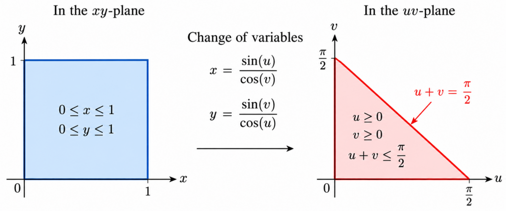
Now comes the surprising part. Introduce new variables u and v by
$x = \frac{\sin (u)}{\cos (v)}, y = \frac{\sin (v)}{\cos (u)} .$
The square
$0 \leq x \leq 1, 0 \leq y \leq 1$
corresponds to the triangular region
$u \geq 0, v \geq 0, u + v \leq \frac{π}{2} .$
To see where the last boundary comes from, notice that
$x \leq 1 \Leftrightarrow \sin (u) \leq \cos (v) \Leftrightarrow u + v \leq \frac{π}{2},$
and the condition on y gives the same inequality.

The Jacobian

We compute
$\frac{\partial x}{\partial u} = \frac{\cos (u)}{\cos (v)}, \frac{\partial x}{\partial v} = \frac{\sin (u) \sin (v)}{{\cos (v)}^{2}} .$
Similarly,
$\frac{\partial y}{\partial u} = \frac{\sin (u) \sin (v)}{{\cos (u)}^{2}}, \frac{\partial y}{\partial v} = \frac{\cos (v)}{\cos (u)} .$
After simplifying the determinant, the Jacobian is
$\frac{\partial (x, y)}{\partial (u, v)} = 1 - x^{2} y^{2} .$
This is exactly the expression that appears in the denominator of our original integral. Therefore,
$\frac{d x d y}{1 - x^{2} y^{2}} = d u d v .$
The complicated-looking integrand has completely disappeared.

The integral becomes an area

Our double integral is now simply
$I = \int_{0}^{\frac{π}{2}} \int_{0}^{\frac{π}{2} - u} d v d u .$
Geometrically, this is the area of a right triangle whose two perpendicular sides both have length
$\frac{π}{2}$
Therefore,
$I = \frac{1}{2} \cdot \frac{π}{2} \cdot \frac{π}{2} = \frac{π^{2}}{8} .$
We have proved that
$1 + \frac{1}{3^{2}} + \frac{1}{5^{2}} + \frac{1}{7^{2}} + \dots = \frac{π^{2}}{8} .$
Recovering the full series

Let
$T = \sum_{n = 1}^{\infty} \frac{1}{n^{2}} .$
Split the series into its odd and even terms. The odd terms have sum
$\frac{π^{2}}{8}$
while the even terms have sum
$\frac{1}{2^{2}} + \frac{1}{4^{2}} + \frac{1}{6^{2}} + \dots = \frac{1}{4} T .$
Consequently,
$T = \frac{π^{2}}{8} + \frac{1}{4} T .$
Thus,
$\frac{3}{4} T = \frac{π^{2}}{8},$
and finally,
$T = \frac{π^{2}}{6} .$
Why this proof is remarkable

We started with an infinite series involving nothing but reciprocals of squares. We then represented part of that series by a double integral over a square. A carefully chosen trigonometric change of variables transformed the square into a triangle and, at the same time, made the integrand disappear.

The infinite series was therefore reduced to the area of a triangle:
$\frac{1}{2} \cdot \frac{π}{2} \cdot \frac{π}{2} = \frac{π^{2}}{8} .$
From there, separating the odd and even terms gives the celebrated result
$\sum_{n = 1} \frac{1}{n^{2}} = \frac{π^{2}}{6} .$
It is a striking example of how an infinite series, a double integral, a trigonometric substitution, and a simple geometric area can all describe the same number.

Another Problem Where Two Dimensions Help

The double-integral proof of the Basel sum illustrates a powerful mathematical idea: sometimes a problem becomes easier when we move to a higher dimension.

One of the most beautiful examples is the Gaussian integral. A one-dimensional integral that resists ordinary antiderivative methods becomes accessible after it is squared and transformed into a two-dimensional integral.

Continue exploring: The Gaussian Integral and Beyond: From e^(-x²) to a Family of Integrals

Long before Euler solved the Basel problem, ancient Greek mathematicians had developed ingenious geometric methods for evaluating infinite sums. In particular, Archimedes used areas of triangles to establish a remarkable infinite series identity. Discover his method in How the Ancient Greeks Summed Infinite Series Without Calculus .

September 28, 2026

When Does x^(1/x) Take the Same Value Twice?

We begin with a simple equality:

2^{\frac{1}{2}} = 4^{\frac{1}{4}} .

The problem

Consider the function $f (x) = x^{\frac{1}{x}}, x > 0 .$ The equality above shows that this function can take the same value at two distinct positive real numbers.

x^{\frac{1}{x}} = y^{\frac{1}{y}}, x \neq y, x > 0, y > 0 .

Prove that infinitely many such pairs exist, and describe all of them.

Solution

Consider the function $f (x) = x^{\frac{1}{x}}$ on $[1, \infty) .$ It increases until $x = e$ and then decreases toward $1 .$ Thus, every horizontal line strictly between $1$ and the maximum intersects the graph twice.

A horizontal line meets the graph twice. Here it gives the approximate pair

(1.471, 7.857) .

A parametrization of all pairs

We now describe all the solutions. Assume first that $x < y$ and set

t = \frac{y}{x} > 1 .

Then

y = t x .

Taking logarithms of $x^{\frac{1}{x}} = y^{\frac{1}{y}}$ gives

\frac{\ln x}{x} = \frac{\ln (t x)}{t x} .

Multiplying by tx, we obtain

t \ln x = \ln x + \ln t .

Therefore,

(t - 1) \ln x = \ln t,

and hence

x = t^{\frac{1}{t - 1}} .

Since y = tx, it follows that

y = t^{\frac{t}{t - 1}} .

Thus, all solutions with $x < y$ are given by

(x, y) = (t^{\frac{1}{t - 1}}, t^{\frac{t}{t - 1}}), t > 1 .

Conversely, direct substitution shows that every $t > 1$ produces a solution. Therefore, this parametrization gives every distinct pair with the smaller number written first. Reversing the two entries gives the solutions with $x > y .$ Since there are infinitely many choices of $t > 1,$ there are infinitely many such pairs.

A Few Examples

Choosing $t = \frac{n + 1}{n}, n = 1, 2, 3, \dots,$ gives the infinite family of rational solutions

(x, y) = ({(\frac{n + 1}{n})}^{n}, {(\frac{n + 1}{n})}^{n + 1}) .

Examples from the rational family
n	t	x	y
1	2	2	4
2	3/2	9/4	27/8
3	4/3	64/27	256/81
4	5/4	625/256	3125/1024

Approaching e

These rational solutions approach $e$ from opposite sides. Indeed, if

x_{n} = {(1 + \frac{1}{n})}^{n}, y_{n} = {(1 + \frac{1}{n})}^{n + 1},

then

x_{n} ↑ e and y_{n} ↓ e .

Thus, the smaller number in each pair approaches $e$ from below, while the larger number approaches $e$ from above.

Another Same-Value Problem

The function $x^{1 / x}$ is not the only familiar-looking function that can take the same value at different inputs. A related question leads to a very different kind of equation.

Continue exploring: When Does x cos(x) Take the Same Value Twice?

September 21, 2026

Tag: calculus

How the Ancient Greeks Summed Infinite Series Without Calculus

1. Zeno and infinitely many steps

2. A square proves a geometric series

3. Archimedes’ quadrature of the parabola

Why does every generation shrink by a factor of four?

4. Why exhaustion proves the result

5. Another area series: thirds

6. Why the harmonic series behaves differently

7. From Greek geometry to calculus

Discovery problems

Solutions (click to reveal)

Historical sources

Kepler’s Laws: How Calculus Explains Planetary Motion

1. Three laws, one mathematical story

2. Newton’s inverse-square force and the orbit equation

3. Kepler’s Second Law: why equal areas take equal times

4. Kepler’s Third Law from the area of an ellipse

5. Worked example: the orbital period of Mars

6. Why a geostationary satellite stays over one point

7. Beyond Kepler: orbital energy and the limits of the model

Discovery problems

Problem 1. How much faster at perihelion?

Problem 2. A planet around a heavier star

Problem 3. Escape velocity

Problem 4. Different shapes, same period

Solutions (open only after trying the problems)

Further connections

A Surprising Improper Integral: Why the Integral of sin(ax)/x Is Always π/2

A Surprising Improper Integral

The Main Idea: Add a Damping Factor

Evaluating the Easier Integral

Recovering F(t)

Removing the Damping

Why Does the Answer Not Depend on a?

What If a Is Zero or Negative?

One Important Detail: The Integral Is Not Absolutely Convergent

A Useful Lesson

Another Surprise from an Improper Integral

From the Dirichlet Integral to the Gaussian Integral

Proving 1 + 1/4 + 1/9 + ⋯ = π²/6 with a Double Integral

Start with the odd terms

Turn the series into a double integral

The key change of variables

The Jacobian

The integral becomes an area

Recovering the full series

Why this proof is remarkable

Another Problem Where Two Dimensions Help