Optimization – Elite Math Program

Is the Brachistochrone Still a Cycloid Underwater?

One of the most beautiful problems in calculus asks:

What path allows an object, starting from rest, to travel between two points under gravity in the least possible time?

The shortest path is a straight line. But the fastest path is not. In the classical brachistochrone problem, the answer is a cycloid.

But there is an assumption hidden inside this famous result: there is no resistance.

What happens if the object moves through a fluid? Is the fastest path in water, oil, or another viscous medium still a cycloid?

The answer is no longer universal. Once resistance is present, the optimal path depends on the law of motion itself.

1. The Classical Brachistochrone

Suppose an object starts from rest and moves under gravity without friction. Let y measure vertical distance downward from the starting point.

Conservation of energy gives

\frac{1}{2} m v^{2} = m g y .

Therefore

v = \sqrt{2 g y} .

If s denotes distance measured along the curve, then speed is

v = \frac{d s}{d t} .

Therefore

d t = \frac{d s}{v} .

The total travel time is consequently

T = \int \frac{d s}{\sqrt{2 g y}} .

For a curve written as y = y(x),

d s = \sqrt{1 + {\frac{d y}{d x}}^{2}} d x .

Thus

T = \int \frac{\sqrt{1 + {\frac{d y}{d x}}^{2}}}{\sqrt{2 g y}} d x .

Minimizing this integral leads to the cycloid.

2. The Exact Cycloid

With y positive downward, the cycloid can be parametrized as

x (θ) = a (θ - \sin (θ)),

y (θ) = a (1 - \cos (θ)) .

The constants are determined by the endpoint.

The cycloid illustrates the central idea behind the brachistochrone. The curve initially descends very steeply. Although this makes the path longer than a straight line, the object gains speed quickly and then uses that speed during the remainder of the trip.

3. What Changes When There Is Resistance?

The classical derivation relies on conservation of mechanical energy. With drag, mechanical energy is continually dissipated.

Consequently, the speed can no longer be determined from height alone. Two objects arriving at the same height along two different paths may have different speeds because they have experienced different histories of drag.

This destroys the simple relation

v = \sqrt{2 g y} .

Now the path and the velocity must be determined together.

4. Linear Drag

A particularly useful mathematical model assumes that the drag force is proportional to speed:

F_{D} = b v .

For a small sphere in the Stokes regime,

b = 6 π μ R,

where μ is the dynamic viscosity and R is the radius of the sphere.

Let s denote arc length along the unknown path. Since

v = \frac{d s}{d t},

the tangential equation of motion is

m \frac{d v}{d t} = m g \frac{d y}{d s} - b v .

Using

\frac{d v}{d t} = \frac{d v}{d s} \frac{d s}{d t} = v \frac{d v}{d s}

we obtain

m v \frac{d v}{d s} = m g \frac{d y}{d s} - b v .

5. What Are We Minimizing?

The quantity we want to minimize is the total travel time. By definition,

v = \frac{d s}{d t} .

Solving for the small amount of time required to travel the distance ds gives

d t = \frac{d s}{v} .

Therefore, for a path of total length S,

T = \int_{0}^{S} \frac{d s}{v} .

In words,

time = distance / speed.

The important difference from the classical brachistochrone is that, in the presence of drag, the speed v is not determined by height alone. It depends on how the object arrived at its current position.

Thus the viscous brachistochrone problem is to find a path and its corresponding velocity that satisfy the equation of motion while making the total travel time as small as possible.

6. Buoyancy

If the object is immersed in a fluid, buoyancy can also be included. For a body of density ρ_s in a fluid of density ρ_f, the effective downward acceleration is

g_{eff} = g (1 - \frac{ρ_{f}}{ρ_{s}}) .

In the equation of motion, g can then be replaced by g_eff.

7. Water Does Not Automatically Mean Linear Drag

There is an important physical qualification. Stokes’ linear drag law applies only in an appropriate low-Reynolds-number regime.

The Reynolds number is

Re = \frac{ρ v L}{μ} .

At higher Reynolds numbers, a quadratic drag model is often more appropriate:

F_{D} = \frac{1}{2} ρ_{f} C_{D} A v^{2} .

If

k = \frac{1}{2} ρ_{f} C_{D} A,

then the corresponding tangential equation is

m v \frac{d v}{d s} = m g \frac{d y}{d s} - k v^{2} .

So there is no single mathematical object called the underwater brachistochrone. The answer depends on the object, the fluid, and the appropriate drag law.

8. A Numerical Example

Let us compare two minimum-time paths having the same endpoints:

(0, 0) and (3, 2) .

As before, y is measured downward.

Case A: No Drag

For the classical cycloid,

x = a (θ - \sin (θ)),

y = a (1 - \cos (θ)) .

The endpoint conditions give approximately

θ_{f} \approx 3.068777, a \approx 1.001327 .

Selected points on the exact cycloid are:

θ	x	y
0.0000	0.0000	0.0000
0.3069	0.0048	0.0468
0.6138	0.0379	0.1828
0.9206	0.1248	0.3952
1.2275	0.2862	0.6643
1.5344	0.5358	0.9649
1.8413	0.8788	1.2689
2.1481	1.3120	1.5479
2.4550	1.8235	1.7758
2.7619	2.3944	1.9313
3.0688	3.0000	2.0000

Case B: Linear Drag

Now keep the same endpoints but introduce linear resistance with

\frac{b}{m} = 1.0 s^{- 1},

and take

g = 9.81 \frac{m}{s^{2}} .

This is a mathematical linear-drag example. We do not label it “water” or “oil,” because identifying a real fluid requires checking which drag law is physically appropriate.

The unknown curve can be approximated numerically by short segments. For each candidate path, the equation of motion is integrated along the path, the travel time is computed, and the intermediate heights are varied to reduce that time.

Selected points from the numerical minimum-time path are:

x	y
0.000	0.000
0.300	0.581
0.600	0.913
0.900	1.181
1.200	1.406
1.500	1.595
1.800	1.749
2.100	1.870
2.400	1.955
2.700	1.997
3.000	2.000

9. Something Unexpected Happens

It is tempting to imagine that adding resistance simply moves the entire brachistochrone to one side of the classical cycloid.

The numerical example shows that this is not what happens.

For comparison, evaluating the classical cycloid at the same horizontal positions gives approximately:

x	Linear-drag y	Cycloid y
0.0	0.000	0.000
0.3	0.581	0.684
0.6	0.913	1.029
0.9	1.181	1.285
1.2	1.406	1.484
1.5	1.595	1.643
1.8	1.749	1.767
2.1	1.870	1.863
2.4	1.955	1.932
2.7	1.997	1.978
3.0	2.000	2.000

At x = 1.8, the linear-drag path has y approximately 1.749, while the cycloid has y approximately 1.767.

But at x = 2.1, the linear-drag path has y approximately 1.870, while the cycloid has y approximately 1.863.

Therefore the two curves cross somewhere between these positions.

This is a useful warning against relying only on intuition. Resistance does not merely shift the classical cycloid uniformly upward or downward. It changes the optimization problem itself and can change the shape in a more subtle way.

10. Why Does Drag Change the Answer?

In the frictionless problem, speed gained early is retained. This makes a steep initial descent extremely valuable.

With drag, there is a competing effect. Descending early still produces speed, but resistance continually removes energy. Speed acquired early is therefore not as valuable as it is in the frictionless problem.

The optimal curve must balance:

gaining speed quickly by descending,
the extra distance caused by that descent, and
the continual loss of energy to resistance.

That competition produces a different minimum-time path.

11. There Is No Single “Brachistochrone in Water”

This is perhaps the most important physical lesson.

Changing the medium can change the viscosity, density, buoyancy, Reynolds number, drag coefficient, and even the mathematical form of the drag law. Changing the size or shape of the moving object can do the same.

Therefore asking

“What is the brachistochrone in water?”

does not completely specify the problem.

A more precise question is:

For this object, in this fluid, under this drag law, what path minimizes the travel time?

12. The Bigger Lesson

The classical brachistochrone is famous because the answer is unexpectedly beautiful: a cycloid.

But there is an even broader lesson hiding behind it.

The fastest path is not determined by geometry alone. It depends on the law of motion.

With no resistance, the answer is a cycloid. With viscous resistance, the speed remembers the history of the path, and the optimization problem changes. For other drag laws, it changes again.

So perhaps the more interesting question is not

“What is the fastest curve?”

but rather

“What physical laws make a particular curve the fastest?”

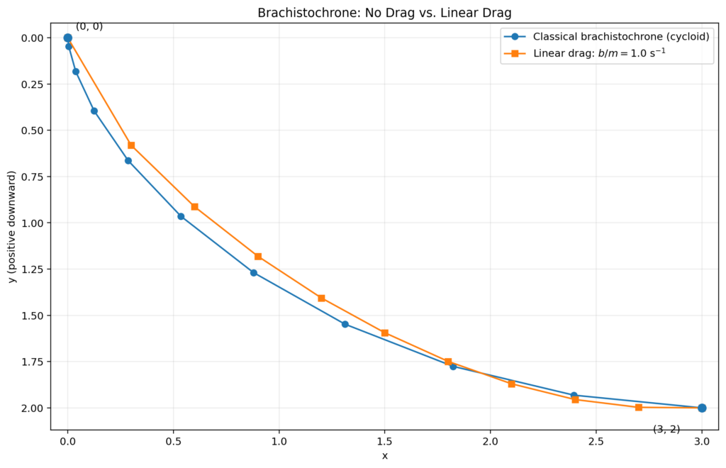
Classical cycloid and numerical linear-drag brachistochrone from (0, 0) to (3, 2), showing the two optimal paths crossing.

Another example where the mathematics of motion produces a surprising result is my related-rates problem about a sliding ladder: is it safer to slide or jump?

October 4, 2026

How Do You Fit a Cylinder to Thousands of Points in Real Time?

Several years ago, I was given a practical geometry problem:

Given thousands of measured points in three-dimensional space, find the cylinder that best fits them.

There was an additional requirement that made the problem much more interesting. The calculation had to be fast enough to operate in real time.

This meant that simply defining a mathematically reasonable fitting problem was not enough. The equations had to be arranged so that thousands of data points could be processed efficiently, the derivatives could be evaluated quickly, and each optimization step would require solving only a very small system of equations.

The resulting method combines geometry, calculus, least squares, and the Gauss–Newton method.

The Geometry of a Cylinder

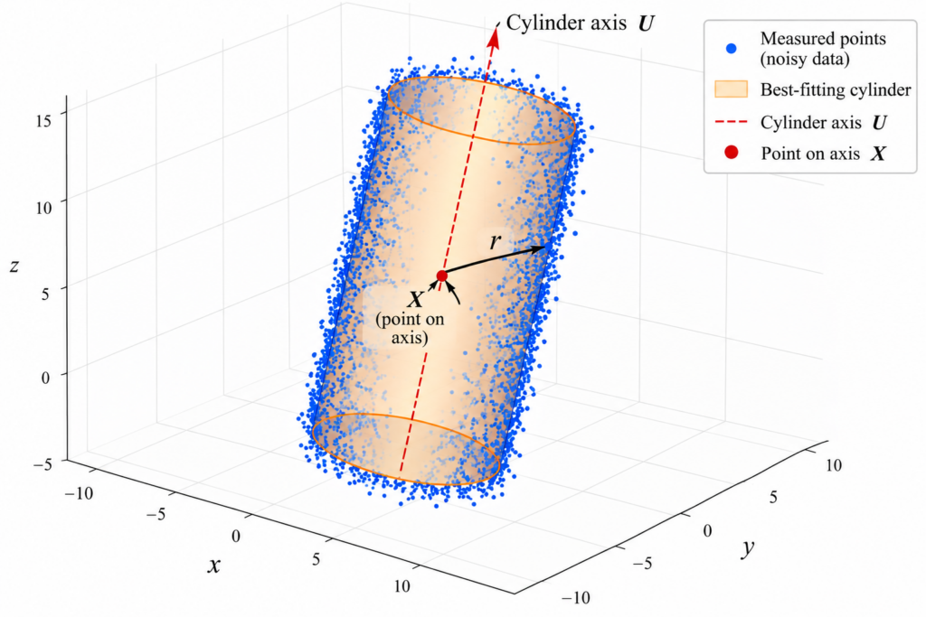
Suppose that

X = {(x_{1}, x_{2}, x_{3})}^{T}

is a point on the axis of a cylinder, and

U = {(u_{1}, u_{2}, u_{3})}^{T}

is a vector pointing along the axis.

Let $P$ be a point on the surface of the cylinder.

The defining geometric property is simple:

The perpendicular distance from every point on the cylinder to its axis is the radius $r$ .

Distance from a Point to the Axis

Consider the vector

P - X .

Part of this vector points along the cylinder axis, while the remaining part is perpendicular to the axis.

If $α$ is the angle between $P - X$ and $U$ , then

‖ P - X ‖ sin α = r .

Squaring gives

{‖ P - X ‖}^{2} {sin α}^{2} = r^{2} .

The dot product gives

{({(P - X)}^{T} U)}^{2} = {‖ P - X ‖}^{2} {‖ U ‖}^{2} {cos α}^{2} .

Combining these relations eliminates the angle completely and gives

{‖ P - X ‖}^{2} - \frac{{({(P - X)}^{T} U)}^{2}}{{‖ U ‖}^{2}} = r^{2} .

This is the equation we need.

The first term measures the squared distance from $X$ to $P$ . The fraction subtracts the squared component parallel to the axis. What remains is exactly the squared perpendicular distance to the axis.

Turning the Geometry into a Residual

Measured points will not lie exactly on a perfect cylinder.

For a measured point $P$ , define

R (P) = {‖ P - X ‖}^{2} - \frac{{({(P - X)}^{T} U)}^{2}}{{‖ U ‖}^{2}} - r^{2} .

For a point exactly on the cylinder,

R (P) = 0 .

For a noisy measured point, the residual will usually be nonzero.

Reducing the Number of Unknowns

At first the cylinder appears to have seven parameters: three coordinates for a point on its axis, three coordinates for the axis direction, and the radius.

But there is redundancy.

Moving the reference point $X$ along the axis does not change the cylinder. Also, multiplying $U$ by a nonzero constant does not change its direction.

Assuming the cylinder axis is not parallel to the $(x_{1}, x_{2})$ plane, choose

X = {(x_{1}, x_{2}, 0)}^{T}, U = {(u_{1}, u_{2}, 1)}^{T} .

Now the entire cylinder is described by only five unknown numbers:

S = {(x_{1}, x_{2}, u_{1}, u_{2}, r)}^{T} .

Two numbers locate the axis, two determine its direction, and one gives the radius.

From Geometry to Least Squares

Suppose our measuring system produces $m$ points:

P_{1}, P_{2}, \dots, P_{m} .

Each point produces a residual $R_{j}$ .

We find the best-fitting cylinder by minimizing

f (S) = \frac{1}{2} \sum_{j = 1}^{m} R_{j}^{2} .

This is a nonlinear least-squares problem.

Why the Derivatives Matter

Because the calculation had to run quickly, I derived the residual derivatives analytically.

For each measured point, we need derivatives with respect to the five unknown parameters:

\nabla R = (\frac{\partial R}{\partial x_{1}}, \frac{\partial R}{\partial x_{2}}, \frac{\partial R}{\partial u_{1}}, \frac{\partial R}{\partial u_{2}}, \frac{\partial R}{\partial r}) .

The formulas contain several repeated expressions. In an implementation, there is no reason to calculate the same quantity over and over.

For example, define

q = \frac{(p_{1} - x_{1}) u_{1} + (p_{2} - x_{2}) u_{2} + p_{3}}{u_{1}^{2} + u_{2}^{2} + 1} .

Then several derivative formulas become much shorter and faster to evaluate.

This may look like a minor algebraic simplification on paper. In a real-time numerical algorithm that evaluates the same expressions thousands of times, such simplifications matter.

The Jacobian

Collect all the residuals into the vector

E = {(R_{1}, R_{2}, \dots, R_{m})}^{T} .

The Jacobian $J$ has one row for every measured point and one column for every unknown parameter.

Therefore,

J is an m \times 5 matrix.

Gauss–Newton

The least-squares objective can be written compactly as

f = \frac{1}{2} {‖ E ‖}^{2} .

Its gradient is

\nabla f = J^{T} E .

Gauss–Newton approximates the Hessian by

\nabla^{2} f \approx J^{T} J .

At each iteration, instead of solving the original nonlinear problem from scratch, we solve

J^{T} J G = - J^{T} E .

The vector $G$ tells us how to change the current estimate of the cylinder.

Why Thousands of Points Are Not as Bad as They Sound

This is the computational feature that makes the method especially attractive.

Suppose the measuring system gives us 10,000 points.

Then $J$ has 10,000 rows.

But it still has only five columns.

Therefore,

J^{T} J

is only a

5 \times 5

matrix.

And

J^{T} E

contains only five numbers.

So although every iteration uses information from thousands of measured points, the linear system that determines the next step has only five unknowns.

That is a very useful structure for a real-time calculation.

Do Not Always Take the Full Step

A Gauss–Newton direction tells us which way to move, but taking the entire step is not always wise.

Write the update as

S_{k + 1} = S_{k} + a_{k} G_{k}, 0 < a_{k} \leq 1 .

The step length is chosen adaptively. Start with $a_{k} = 1$ and reduce it if necessary until the new point produces a sufficient decrease in the objective function.

In practice, the full step can often be accepted, but the line search gives the algorithm additional protection when the current estimate is not yet close to the solution.

When Do We Stop?

At a minimum we expect

\nabla f = 0 .

Numerically, we stop when

‖ \nabla f ‖ < ε,

where $ε$ is a small tolerance.

There is no benefit in demanding far more numerical precision than the data and the computer arithmetic can support. An unnecessarily small tolerance can even create numerical difficulties.

Did It Work?

Yes.

This was not a numerical example invented after the fact. The cylinder fitting problem came from a real application, and the algorithm had to work fast enough for real-time use.

The implementation worked extremely well.

What I found especially satisfying was that the final algorithm was built from familiar mathematical ingredients:

geometry → least squares → calculus → Gauss–Newton → real-time computation.

The important part was arranging those ingredients in the right way.

From Cylinders to Cones

A cylinder has constant radius. Once this fitting method works, a natural question is:

What happens if the radius changes as we move along the axis?

That leads to a cone.

The cone-fitting problem requires one additional parameter—the opening angle—and the derivatives become more complicated. But the central strategy remains the same:

choose an efficient geometric residual → derive its Jacobian → form a nonlinear least-squares problem → solve it with Gauss–Newton.

That will be the subject of the next post.

The Larger Lesson

There is an important distinction between solving a mathematical problem and solving it in a form that is useful in practice.

With 10,000 measured points, the original problem sounds large. But the geometry allows the unknown cylinder to be represented by only five parameters. Gauss–Newton then converts each iteration into a small five-variable linear problem.

This is one of the recurring ideas in applied mathematics:

A good mathematical formulation can be as important as the algorithm itself.

When the formulation is right, a problem involving thousands of three-dimensional measurements can become small enough to solve in real time.

A Closely Related Fitting Problem

Cylinder fitting is only one version of the real-time surface-fitting problem. A closely related challenge arises when the measured surface is a cone rather than a cylinder.

The change in geometry leads to a different mathematical problem, but the objective is the same: use the structure of the surface to obtain an accurate fit quickly enough for practical real-time computation.

Continue exploring: How Do You Fit a Cone to Thousands of Points in Real Time?

October 1, 2026

How Do You Fit a Cone to Thousands of Points in Real Time?

Several years ago, I was given an applied mathematics problem that sounded simple at first:

Given thousands of measured points in three-dimensional space, find the cone that best fits them.

But there was an additional requirement that changed the problem completely. The calculation had to be fast enough to be used in real time.

It is one thing to describe an optimization problem mathematically. It is another thing to solve it repeatedly, quickly, and reliably while a real system is operating.

The solution came from combining elementary geometry with nonlinear least squares and the Gauss–Newton method.

The Geometric Problem

Suppose a collection of measured points

P_{1}, P_{2}, \dots, P_{m}

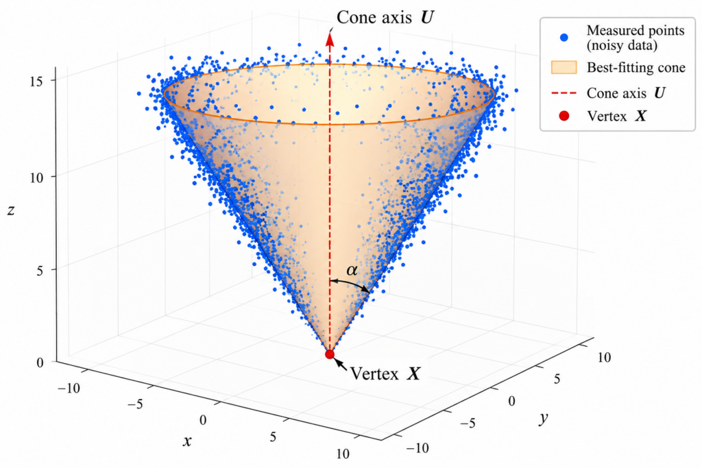
lies close to the surface of an unknown right circular cone.

We want to determine three things:

the vertex of the cone, the direction of its axis, and its opening angle.

Let

X = (x_{1}, x_{2}, x_{3})

be the vertex, let $U$ point along the axis, and let $α$ be the half-angle of the cone.

If $P$ lies exactly on the cone, then the vector

P - X

makes angle $α$ with the cone axis.

The dot-product formula for the angle between two vectors therefore gives

{({(P - X)}^{T} U)}^{2} = {‖ P - X ‖}^{2} {‖ U ‖}^{2} {cos α}^{2} .

This one equation contains the geometry of the cone.

Turning Geometry into an Error

Measured data will not lie exactly on a perfect cone. There will be noise, measurement error, and small deviations from the ideal surface.

So instead of asking whether a point satisfies the cone equation exactly, we measure how far it is from satisfying the equation.

Define the residual

R (P) = {‖ P - X ‖}^{2} {cos α}^{2} - \frac{{({(P - X)}^{T} U)}^{2}}{{‖ U ‖}^{2}} .

For a point exactly on the cone,

R (P) = 0 .

For a measured point near the cone, the residual will generally be nonzero.

Why Use This Residual?

There is an important practical point here.

One could try to calculate the exact shortest geometric distance from every measured point to the cone. But when thousands of points must be processed repeatedly in real time, the computational form of the problem matters.

The residual above is obtained directly from the cone equation. It can be evaluated using additions, multiplications, dot products, and a few simple functions.

This was exactly what was needed for the application: a mathematical description that could be differentiated explicitly and evaluated rapidly.

Six Unknown Parameters

The direction of the axis does not depend on the length of $U$ . Multiplying the axis vector by a nonzero constant gives the same axis.

Assuming the axis is not parallel to the $(x_{1}, x_{2})$ plane, we can therefore write

U = (u_{1}, u_{2}, 1) .

The entire cone is then described by only six unknown numbers:

S = {(x_{1}, x_{2}, x_{3}, u_{1}, u_{2}, α)}^{T} .

Three numbers locate the vertex, two determine the axis direction, and one determines the cone angle.

From One Point to Thousands of Points

Suppose there are $m$ measured points.

For each point $P_{j}$ , compute a residual $R_{j}$ .

We then look for the cone that minimizes the total squared residual:

f (S) = \frac{1}{2} \sum_{j = 1}^{m} R_{j}^{2} .

This is a nonlinear least-squares problem.

Why Not Just Solve the Equations?

If the measurements were perfect, six carefully chosen points might appear to be enough to determine six unknown parameters.

Real data do not work that way.

Measurements contain noise, and a small collection of points may give a poor estimate. Instead, we can use hundreds or thousands of points simultaneously and find the cone that best fits all of them.

But now the equations are nonlinear. There is no simple matrix formula that immediately gives the answer.

This is where Gauss–Newton enters the story.

The Jacobian

Put all the residuals into one vector:

E = {(R_{1}, R_{2}, \dots, R_{m})}^{T} .

Then

f = \frac{1}{2} {‖ E ‖}^{2} .

The Jacobian $J$ contains the derivatives of every residual with respect to the six cone parameters.

Its $j$ -th row is

J_{j} = (\frac{\partial R_{j}}{\partial x_{1}}, \frac{\partial R_{j}}{\partial x_{2}}, \frac{\partial R_{j}}{\partial x_{3}}, \frac{\partial R_{j}}{\partial u_{1}}, \frac{\partial R_{j}}{\partial u_{2}}, \frac{\partial R_{j}}{\partial α}) .

In the actual implementation, these derivatives were derived analytically rather than estimated numerically.

That requires more work at the beginning, but once the formulas are known, they can be evaluated very efficiently.

The Key Gauss–Newton Approximation

The gradient of the least-squares objective has a particularly simple form:

\nabla f = J^{T} E .

The exact Hessian is

\nabla^{2} f = J^{T} J + \sum_{j = 1}^{m} R_{j} \nabla^{2} R_{j} .

Computing the second term repeatedly is considerably more expensive.

Gauss–Newton makes the approximation

\nabla^{2} f \approx J^{T} J .

This approximation becomes especially natural when the fit is already good, because the residuals $R_{j}$ are then small.

That observation was crucial for a real-time implementation. Instead of constructing the complete second derivative at every iteration, we can work primarily with the Jacobian.

One Iteration

At the current estimate $S_{k}$ , the Gauss–Newton direction $G_{k}$ is obtained by solving

{J_{k}}^{T} J_{k} G_{k} = - {J_{k}}^{T} E_{k} .

Then update the six cone parameters:

S_{k + 1} = S_{k} + a_{k} G_{k} .

Here $0 < a_{k} \leq 1$ is the step length.

Why Use a Line Search?

Taking the full Gauss–Newton step is not always a good idea when the current estimate is still far from the solution.

The implementation therefore reduces the step when necessary until the objective function decreases sufficiently.

In mathematical form, choose the step length so that

f (S_{k} + a_{k} G_{k}) \leq f (S_{k}) + ρ a_{k} {\nabla f_{k}}^{T} G_{k} .

The purpose is simple: do not accept an iteration that moves too aggressively in a direction that fails to improve the fit sufficiently.

The Real-Time Idea

At first glance this may still look like a large calculation. There may be thousands of measured points.

But notice something important.

No matter how many data points we have, there are still only six unknown cone parameters.

The Jacobian may have thousands of rows, but only six columns. The matrix

J^{T} J

is therefore only

6 \times 6 .

Similarly,

J^{T} E

has only six components.

So the data set can be large while the system that must be solved at each Gauss–Newton iteration remains very small.

This is exactly the type of structure one wants to exploit in a real-time numerical algorithm.

Did It Work?

Yes.

This was not an exercise invented to demonstrate Gauss–Newton. I developed the method because the cone-fitting calculation was needed in a real application, and it had to operate in real time.

The implementation worked extremely well.

That experience taught me an important lesson about applied mathematics: the best mathematical formulation is not necessarily the one that looks most sophisticated on paper.

Sometimes the decisive question is:

Can we formulate the problem so that the computer can solve it quickly enough to be useful?

Why the Approximation Works

There is another nice feature of Gauss–Newton.

Recall that the exact Hessian is

\nabla^{2} f = J^{T} J + \sum_{j = 1}^{m} R_{j} \nabla^{2} R_{j} .

As the estimated cone approaches the data, the residuals become small. Consequently, the second term becomes less important and

\nabla^{2} f \approx J^{T} J .

So as the algorithm approaches a good fit, the inexpensive approximation becomes increasingly appropriate.

A Final Check

Although computing the full Hessian at every iteration is expensive, it can still be useful after the optimization has finished.

At the final solution we can evaluate

\nabla^{2} f = J^{T} J + \sum_{j = 1}^{m} R_{j} \nabla^{2} R_{j} .

If its eigenvalues are positive, the Hessian is positive definite and the computed stationary point is a local minimum.

In other words, we use the inexpensive approximation while speed matters, and we can use the more expensive calculation afterward as a check.

The Larger Lesson

The mathematics of this problem can be summarized in one chain:

3D measurements → cone geometry → residuals → least squares → Jacobian → Gauss–Newton → real-time fit.

The cone itself is elementary geometry. Least squares is a classical idea. The derivatives require calculus. Gauss–Newton comes from numerical optimization.

None of these ingredients alone solves the practical problem.

The solution comes from putting them together in a form that a computer can evaluate rapidly.

That is one of the most satisfying aspects of applied mathematics: sometimes a few familiar mathematical ideas, combined in the right way, turn a difficult real-world computation into something that works almost like magic.

A Closely Related Fitting Problem

Fitting a cone to a large cloud of measured points is one example of a broader problem: how can we recover a geometric surface accurately when the computation has to be fast enough for real-time use?

A closely related problem replaces the cone by a cylinder. The geometry changes, but the same practical challenge remains: turn thousands of measurements into a reliable geometric fit without an expensive general-purpose optimization.

Continue exploring: How Do You Fit a Cylinder to Thousands of Points in Real Time?

October 1, 2026

Category: Optimization

Is the Brachistochrone Still a Cycloid Underwater?

1. The Classical Brachistochrone

2. The Exact Cycloid

3. What Changes When There Is Resistance?

4. Linear Drag

5. What Are We Minimizing?

6. Buoyancy

7. Water Does Not Automatically Mean Linear Drag

8. A Numerical Example

Case A: No Drag

Case B: Linear Drag

9. Something Unexpected Happens

10. Why Does Drag Change the Answer?

11. There Is No Single “Brachistochrone in Water”

12. The Bigger Lesson

How Do You Fit a Cylinder to Thousands of Points in Real Time?

The Geometry of a Cylinder

Distance from a Point to the Axis

Turning the Geometry into a Residual

Reducing the Number of Unknowns

From Geometry to Least Squares

Why the Derivatives Matter

The Jacobian

Gauss–Newton

Why Thousands of Points Are Not as Bad as They Sound

Do Not Always Take the Full Step

When Do We Stop?

Did It Work?

From Cylinders to Cones

The Larger Lesson

A Closely Related Fitting Problem

How Do You Fit a Cone to Thousands of Points in Real Time?

The Geometric Problem

Turning Geometry into an Error

Why Use This Residual?

Six Unknown Parameters

From One Point to Thousands of Points

Why Not Just Solve the Equations?

The Jacobian

The Key Gauss–Newton Approximation

One Iteration

Why Use a Line Search?

The Real-Time Idea

Did It Work?

Why the Approximation Works

A Final Check

The Larger Lesson

A Closely Related Fitting Problem